GFD's 100-share Index
Existing calculations of long-term stock market returns in the United States are based upon four primary sources: Smith and Cole (1803-1862), Macaulay (1857-1871) Cowles (1871-1928) and Standard and Poor’s (1928-2017). Unfortunately, these indices have major flaws in them that create biases that researchers have tolerated until now because no one has ever collected historical data on U.S. share prices, corporate actions (dividends and splits) and shares outstanding so accurate price and return indices could be calculated. The current S&P Composite includes data from the Cowles Indices from 1871 until 1927, the 90-share daily S&P Index from January 1928 until February 1957, the 500-share composite that excludes finance stocks until July 1976 and the all-sector 500-share index since July 1, 1976. Global Financial Data has collected data on all major United States exchanges going back to 1791 as well as data on over-the-counter shares since 1865. The data includes not only share price data, but information on corporate actions (dividends and splits) as well as shares outstanding. These data sources enable us to calculate cap-weighted price and return indices for the United States that accurately reflect what an investment in the 100 largest stocks each year would have produced for investors. GFD set up criteria for determining which stocks are included or excluded from its indices. GFD has followed these rules for inclusion: 1) There have to be at least 9 observations per year for each stock and there have to be at least two price changes during each year to warrant inclusion. Otherwise, the stock was excluded due to illiquidity. 2) Dividend data have to be available for each stock in order that both price and return indices can be calculated. A stock may not have paid a dividend during a particular year, but to be included, we had to know the company had passed on paying a dividend during that year. Any shares for which we were unable to find dividend information was excluded. 3) There had to be share outstanding information available so the stock could be included in a capitalization-weighted index 4) Only non-assessable shares were included. A stock was excluded if it imposed assessments on shareholders. Shares that were liquidating assets and were paying liquidating dividends were excluded as well. The index includes all shares that met these criteria from 1791 to 1824, the top 50 shares by capitalization are used from 1825 to1850 and the top 100 shares by capitalization from 1851 to 2017. Although GFD plans to calculate indices that include more than 100 shares in the future, we decided that because the index was capitalization-weighted, a 100-share index would track a 500-share index very closely. The graph below compares the performance of the S&P 100 (green line) and the S&P 500 (black line) between 1976 and 2018. The performance of the two is very similar. The S&P 500 did outperform the S&P 100 by 0.5% per annum, but the returns are close enough to show that a strong correlation exists between the top 100 shares and the top 500 shares. In 2017, the top 100 shares in the S&P 500 represented about 60% of the total capitalization of the S&P 500.

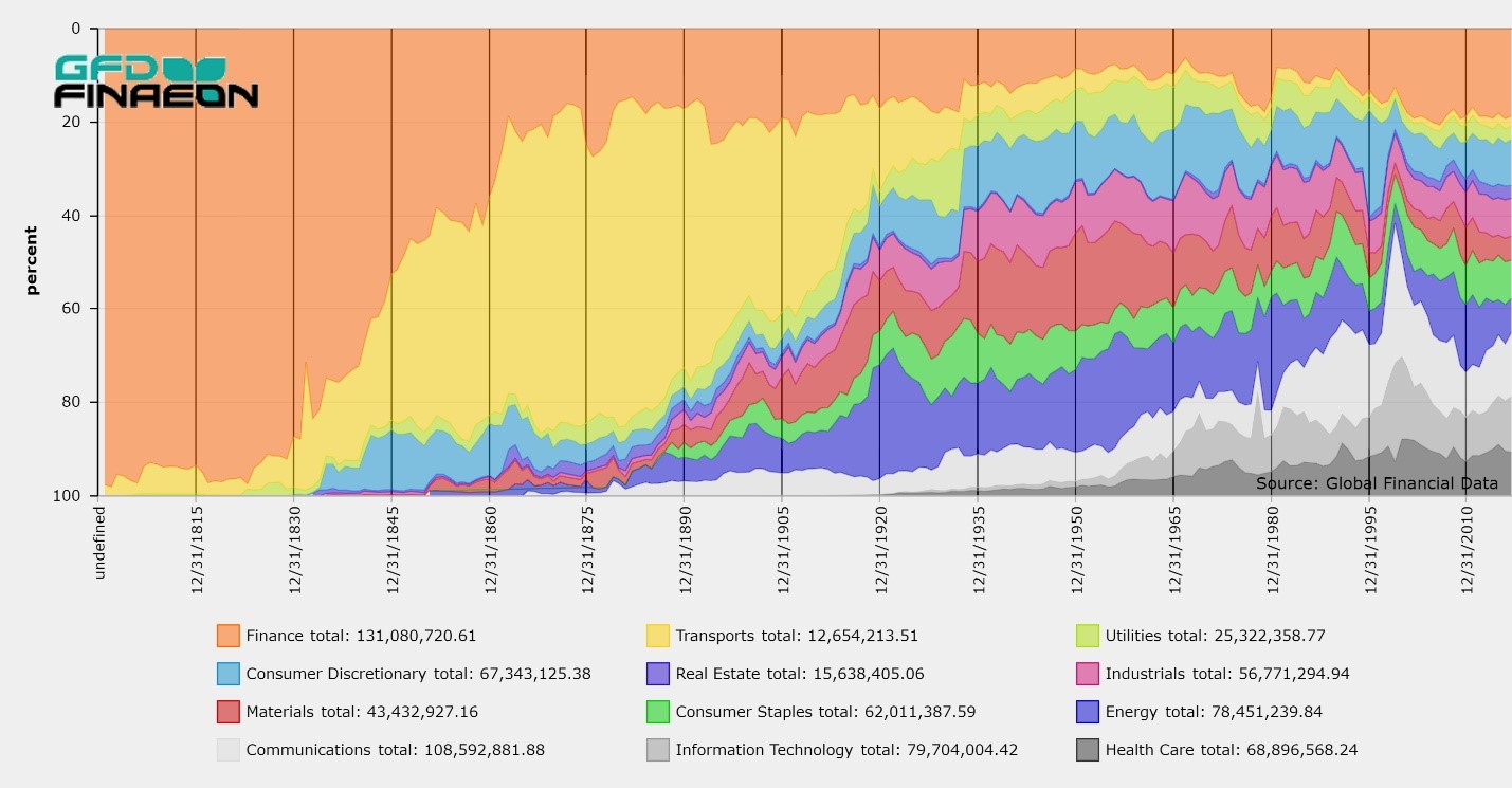
To choose which companies to include, shares were weighted by capitalization during the first month of each year and included if they were among the 100 largest shares in the United States. It was assumed that the stocks were held for the rest of the year, and in January of the next year, the same selection methodology was used to choose which shares to hold for the coming year. Each year, the list of the 100 largest companies was recalculated and a new list of stocks was introduced. For continuity purposes, if a stock missed a year, i.e. the stock was in the top 100 in 1914 and 1916, but not in 1915, the stock was included in the index in 1915 even though this put over 100 stocks in the index. Initially, there were less than 100 shares in the index because of a lack of companies that met the criteria outlined above. There were only 3 companies in 1791, 7 in 1800, 18 in 1810, 25 in 1820 and 50 in 1825. The index included 50 members through 1850 and beginning in 1851, there were 100 shares in the index. The chart below shows the sectoral composition of the GFD-100 index from 1800 until 2017 to cover the period before the introduction of the Cowles indices in 1871. However, the Smith and Cole indices have some major biases in them. The indices use a very limited number of companies, excluding, for example, the first and second Bank of the United States, which represented from 50% to 80% of the overall capitalization of the United States stock market. Consequently, Smith and Cole exclude over half of the U.S. stock market in their indices.

As can be seen, finance stocks (banks and insurance companies) represented over 95% of the capitalization until 1825. After 1825, the transportation sector grew, first with canals and then with railroads. By the 1840s, transports represented over half of the total capitalization, growing to 80% by the 1870s, then shrinking as industrials began to dominate the U.S. stock market. By 1900, industrial stocks represented about 40% of total capitalization with Energy stocks, primarily Standard Oil and its subsidiaries, representing a growing portion of total capitalization. It should be noted that Standard Oil of New Jersey and California (ExxonMobil and Chevron) weren’t included in the Cowles indices until 1918 when Standard Oil listed on the NYSE. By 1918, Standard Oil had grown tenfold in size to become the largest company in the world, yet was not included in any indices because it traded over-the-counter. And as we stated previously, no finance stocks were included in either the Cowles indices or the S&P indices until 1976. Therefore, we feel that the composition of stocks in the GFD indices are more representative of the stocks that were available to investors in the United States than any of the existing indices of United States stocks. To show how the GFD-100 index differs from existing indices of U.S. stocks we will compare the components and performance of the GFD-100 index and other indices.
Survivorship Bias in the Smith and Cole Indices
Currently, no index for U.S. stocks exists prior to 1802 when the Smith and Cole indices begin. Therefore, the GFD-100 index covers data that is currently unavailable from existing indices. The graph below compares the Cole and Smith indices (USCFALLM) with the GFD-100 index (GFUS100MPM) from 1802 until 1845 when Smith and Cole’s Bank and Insurance index was discontinued. As can be seen, the Smith and Cole index outperforms the GFD-100 index; however, in analyzing how the Smith and Cole indices were put together, we discovered that the superior performance was caused by the survivorship bias that Smith and Cole built into their indices.

In Walter B. Smith and Arthur H. Cole, Fluctuations in American Business, 1790-1860, Cambridge: Harvard Univ. Press, 1935, they provided calculations of stock market indices for Banks (1802-1820), Banks and Insurance (1815-1845) and Railroad (1834-1862) shares which have been used to cover the period before the introduction of the Cowles indices in 1871. However, the Smith and Cole indices have some major biases in them. The indices use a very limited number of companies, excluding, for example, the first and second Bank of the United States, which represented from 50% to 80% of the overall capitalization of the United States stock market. Consequently, Smith and Cole exclude over half of the U.S. stock market in their indices. For the dataset of bank stocks from 1802 until 1820, Smith and Cole collected data on 21 bank stocks, 9 insurance shares, 5 bridge and turnpike shares and 3 miscellaneous companies. Smith and Cole based their index on 7 bank stocks which existed during the entire 19-year period from 1802 until 1820, creating a survivorship bias. Banks such as the first Bank of the United States were excluded because they did not survive until 1820. Since Smith and Cole collected no data on shares outstanding, the index was calculated as a geometric mean of the underlying shares. The index is not cap-weighted even though it included only 7 banks. Because Smith and Cole collected no data on dividends, no return index was calculated. Scholars who have attempted to calculate total returns have calculated a dividend yield based upon the yield on government stocks. Jeremy Siegel in his book Stocks for the Long Run, uses a 6.4% dividend between 1802 and 1870. Smith and Cole collected data on 17 bank stocks, 5 canal stocks, 3 gas-light stocks, 19 insurance stocks, 27 rail, 6 miscellaneous and 17 Boston bank shares between 1815 and 1845. From these shares, they chose 6 bank shares and 1 insurance company for the Bank and Insurance index. Again, only stocks that survived the 30-year stretch between 1815 and 1845 were included, once again creating a survivorship bias. Finally, Smith and Cole calculated a railroad index that went from 1834 to 1862. Smith and Cole removed shares that either changed little or were erratic in their behavior. They broke up the data into 8 shares from1834 to 1853 and in several cases, because the data series were incomplete, they “spliced” together some of the series even though they admitted this was a statistical device of “questionable value.” Smith and Cole calculated two rail indices of 8 and 10 shares from 1834 to 1853 and a composite of 18 shares from 1853 to 1862. Finally, they calculated a chain-linked index of railway shares that covered 1834 to 1862 as well as some regional rail indices. A railway index of 25 shares calculated by Frederick R. Macaulay in The Movements of Interest Rates, Bond Yields and Stock Prices in the United States Since 1856, New York: National Bureau of Economic Research, 1938 was used to fill in the gap between 1862 and 1870. The performance of the rail indices is provided below. Although the GFD-100 and Smith and Cole Rail index take divergent paths, they both end up at the same levels over the 28-year period. The GFD Transports outperform the Smith and Cole Railway Index, especially in the 1850s, but the general pattern of their performance at any point in time is similar. The difference lies in the rate of return.

It is unfortunate that the Smith and Cole indices have been the sole source of returns for the United States before 1870. The problem with the Smith and Cole indices are several: 1) they use a limited number of stocks, 2) their selection process creates a survivorship bias that increases returns, 3) calculations are based upon the geometric mean of the shares rather than the capitalization of each share, 4) railway shares are spliced together to provide consistent coverage, and 5) no data on dividends was collected so no total returns could be calculated. As was discussed above, because of the survivorship bias that is inherent in the Cole and Smith indices, one would expect that their indices would outperform the other indices that lack a survivorship bias. The survivorship bias is particularly notable in the exclusion of the second Bank of the United States. After the bank lost its charter from the Federal government in 1836, Stephen Girard took over the bank and privatized it. The bank collapsed during the depression that followed the Panic of 1837, and Bank of the United States stock declined in value from 123 in January 1839 to 3.5 by December 1841. The bank’s capitalization fell from $42 million to $1 million. The GFD-100 index lost almost half of its value as a result. The chart below compares the Smith and Cole/Macaulay index with the GFD-100 index from 1802 until 1871. As can be seen, the survivorship bias enables the Smith and Cole/Macaulay index to outperform the GFD-100 during the entire period. From 1845 on, the Smith and Cole/Macaulay index includes no finance stocks and outperforms the GFD-100 even more. The combination of survivorship bias and exclusion of bank and insurance shares after 1845 causes the GFD-100 to underperform the Smith and Cole/Macaulay index. Because the GFD-100 includes more stocks and is cap-weighted, it provides a better representation of the return shareholders would have received before the introduction of the Cowles indices in 1871.

Limitations of the Cowles Indices
In the 1930s, Cowles created cap-weighted indices for the United States going back to 1871. The Commercial and Financial Chronicle published annual summaries of monthly high and low prices for stocks. The Cowles Commission collected data on shares outstanding and dividends in order to calculate cap-weighted price and total return indices for the United States. The Cowles indices included 44 shares in 1871, 75 in 1880, 88 in 1890, 102 in 1900, 126 in 1910, 243 in 1920 and 450 in 1930. The GFD-100 index included about 100 shares in each of those years. Although the Cowles indices are cap-weighted and include dividends, there are drawbacks to the Cowles indices. In calculating the indices, prices were based upon the average of the high and low prices for each month, not on the closing price of shares in each month. Although this factor affects the volatility of the indices, it should have a minimal impact on the long-term returns of the index. More importantly, the selection of stocks was limited to shares traded on the New York Stock Exchange. This means that bank and insurance shares as well as Standard Oil and other non-NYSE companies are completely excluded from the Cowles indices. Even though Standard Oil began trading in 1882, neither Standard Oil of New Jersey (ExxonMobil) nor of California (Chevron) was included in the Cowles indices until 1918 when they joined the NYSE. At the time, Standard Oil was the largest corporation in the world. The impact of excluding Standard Oil, banks and insurance companies is illustrated below.

Standard Oil (XOM – blue) clearly outperformed the other indices with finance stocks (GFUSBNKINSMPM – green) coming in second. Transports (GFUSTRANSMPM – black) did outperform the Cowles Indices (_SPXD – purple), but the Cowles indices provided the lowest return of the indices in the graph. The graph below looks at the sectoral composition of the Cowles/S&P Broad Composite index from 1871 to 1957 when it was discontinued in favor of the S&P 500. This sector chart can be compared with the sector chart of the GFD-100 provided above. As can be seen, the Cowles/S&P index is missing the finance sector and gives a lower weighting to the Energy sector than the GFD-100 sector chart. This absence is made up by the larger role of transportation (railroad) shares in the index until the 1920s.

The GFD-100 and the S&P 90/500
The S&P 90-share index was introduced on January 1, 1928. It is used as the basis for the S&P Composite through March 1, 1957 when the S&P 500 replaced the S&P 90. Both the GFD-100 and the S&P 90 use a similar number of shares between 1928 and 1957 and as the graph below shows, the two indices track each other very well. The S&P 500 was introduced on March 1, 1957 and excluded finance stocks until July 1, 1976 when 40 finance shares were included in the S&P 500. On April 6, 1988 exact sectoral balances were dropped and the number of industrial, utility, transportation and finance stocks was based purely upon market cap, not on fixed ratios for different sectors. The chart below compares the performance of the GFD-100 and the S&P 90/500 index between 1918 when Standard Oil and Chevron listed on the NYSE and 1976 when finance stocks were added to the index. The correlation between the two indices is strong with the GFD-100 providing a 5.1% annual return between 1918 and 1976 and the S&P Composite providing a 4.7% return during the same period. Although we found reasons for the difference in the performance of the GFD-100 and the Smith and Cole/Cowles indices between 1802 and 1918, the similarity in composition between the GFD-100 and the S&P Indices has generated quite similar returns between 1918 and 1976.

Total Returns
Until now, we have only looked at the return to the price indices for the GFD-100 and the S&P Composite. Of course, shareholders receive dividends in addition to capital gains and historically, shareholders have received a higher return from dividends than from capital gains. Until now, no one has ever measured the dividends shareholders received before 1871. GFD’s calculations show that before 1871, U.S. shareholders on average received no capital gains. This means that 100% of shareholder return came from dividends. GFD has collected historical data on the dividends that were paid by thousands of companies in order that we could accurately calculate the dividends that shareholders received. A comparison of the yields on the S&P Cowles Composite and the GFD-100 is provided below. You can generally observe that the dividend yield declined between 1791 and 1820, rose from 1820 until 1870, then declined for the rest of the 1800s. The dividend yield shows similar behavior in the GFD-100 and the S&P Composite between 1871 and 2017. The dividends for the S&P Composite appear to be more volatile than the yields on the GFD-100 between 1871 and 1980. The reason for this lies in the different methodology used to calculate the dividend yield. S&P/Cowles collected data on annual dividends through 1935 and quarterly thereafter. The S&P dividend yield was calculated by dividing the annual dividends that were “paid” to shareholders by the price of the S&P Composite. Consequently, a large decline or rise in the S&P Composite index caused a spike in the dividend yield. Data for the GFD-100 dividend yield is calculated on an ongoing basis from month to month when the dividends are “paid” to the component companies on the ex-date, reducing the volatility in the dividend yield. Nevertheless, the dividend yield of the GFD-100 and the S&P Cowles Composite follow each other fairly closely. With this dividend data, we can calculate the total return to U.S. stocks over the entire period covered. No estimates based upon the yield on government bonds is needed. The total return from the GFD-100 and the S&P Composite are illustrated below. As can be seen, over the long-term, the differences between the two indices is small. The Smith/Cole/Cowles data outperform the GFD-100 in the early 1800s because of the survivorship bias inherent in the Smith and Cole data. However, the exclusion of over-the-counter shares (Standard Oil and finance stocks) by Cowles between 1871 and 1918 allows the GFD-100 to “catch up” with the Composite data. The two indices then track each other closely from 1918 until 1976 when S&P introduced bank and insurance shares into the S&P 500 Composite.

We can provide actual data on the total returns to the two indices in order that the two sets of indices can be compared directly. The table below shows the returns of the GFD-100 and the S&P Composite between 1802 and 2017. Annual capital gains for the GFD data and the S&P data are provided in the first two columns. Total Returns including reinvested dividends are provided in the next two columns and the dividends that were paid are compared in the last two columns. The returns are very similar over the 215 years for which both indices have data with capital gains of 3.57% per annum for the GFD-100 and 3.46% for the Cowles/S&P Composite. After dividends are added and total returns are calculated, similar numbers result. The GFD-100 provided a total return of 8.75% per annum and the Smith/Cole/Cowles/S&P Composite provided an 8.38% total return between 1802 and 2017. The dividends we interpolated between 1802 to 1870 was calculated as the yield on government bonds plus 1% yielding an annual dividend of 5.76%. If the dividend yield of 6.42% that we actually calculated between 1802 and 1870 were used, the total return to the S&P Composite would equal 8.67% between 1802 and 2017 which is close to the GFD-100 annual return of 8.75%. The period from 1802 until 2017 is also divided into a pre-Cowles period from 1802 until 1870 when Smith and Cole/Macaulay were the only source for indices, the period from 1871 to 1918 when Standard Oil was excluded from the index, and 1918 until 1976 when S&P calculated the index, but excluded finance shares.
Table 1 Comparison of Returns to GFD-100 and Cowles/S&P Composite
| SPX | GFD | SPX | ||||
|---|---|---|---|---|---|---|
| Period | GFD Nominal | Nominal | GFD TR | SPX TR | Dividends | Dividends |
| 1802-1870 | -0.03 | 1.33 | 6.39 | 7.17 | 6.42 | 5.76 |
| 1871-1918 | 2.15 | 0.93 | 7.75 | 5.88 | 5.48 | 4.9 |
| 1918-1976 | 5.2 | 4.82 | 9.63 | 9.9 | 4.21 | 4.84 |
| 1802-1976 | 2.19 | 2.36 | 7.79 | 7.67 | 5.48 | 5.19 |
| 1802-2017 | 3.57 | 3.46 | 8.75 | 8.38 | 5 | 4.76 |
| 1791-2017 | 3.32 | 8.54 | 5.05 |
A decade-by-decade comparison of the return to stocks in the GFD-100, bonds in GFD’s U.S. Bond Index, bills in GFD’s US Bill Index and the equity-risk premium is provided below.
Decade-by-Decade Returns to Stocks, Bonds and Bills in the United States
| Decade | Stock Price | Stock Return | Dividends | Bonds | Cash | Equity Premium |
|---|---|---|---|---|---|---|
| 1792-1799 | -3.7 | 2.67 | 6.61 | -0.15 | 5.75 | -2.91 |
| 1800-1809 | 1.35 | 8.01 | 6.57 | 6.03 | 4.96 | 2.91 |
| 1810-1819 | -4.35 | 1.59 | 6.21 | 7.42 | 4.99 | -3.24 |
| 1820-1829 | 0.53 | 5.82 | 5.26 | 5.01 | 3.66 | 2.08 |
| 1830-1839 | -0.95 | 5 | 6.01 | 0.44 | 4.51 | 0.47 |
| 1840-1849 | -0.8 | 6.12 | 6.98 | 6.97 | 4.94 | 1.12 |
| 1850-1859 | -0.58 | 6.65 | 7.27 | 4.67 | 5.01 | 1.56 |
| 1860-1869 | 4.62 | 12.45 | 7.48 | 9.28 | 4.97 | 7.13 |
| 1870-1879 | 2.04 | 8.97 | 6.79 | 5.52 | 3.82 | 4.96 |
| 1880-1889 | 1.19 | 6.27 | 5.02 | 4.16 | 3.01 | 3.16 |
| 1890-1899 | 4.05 | 9.45 | 5.19 | 4.57 | 2.13 | 7.17 |
| 1900-1909 | 6.25 | 11.23 | 4.69 | 0.76 | 3.01 | 7.98 |
| 1910-1919 | -0.69 | 5.5 | 6.23 | 2.22 | 2.62 | 2.81 |
| 1920-1929 | 8.72 | 14.44 | 5.26 | 5.53 | 3.5 | 10.57 |
| 1930-1939 | -3.48 | 0.5 | 4.12 | 6.32 | 0.27 | 0.23 |
| 1940-1949 | 3.43 | 8.21 | 4.62 | 2.25 | 0.58 | 7.59 |
| 1950-1959 | 13.67 | 18.3 | 4.07 | 0.70 | 2.16 | 15.80 |
| 1960-1969 | 3.82 | 6.83 | 2.90 | 1.28 | 4.4 | 2.33 |
| 1970-1979 | 2.14 | 6.12 | 3.90 | 4.09 | 6.71 | -0.55 |
| 1980-1989 | 12.94 | 18.14 | 4.60 | 15.54 | 7.96 | 9.43 |
| 1990-1999 | 19.78 | 22.65 | 2.40 | 7.20 | 4.52 | 17.35 |
| 2000-2009 | -1.66 | 0.16 | 1.85 | 5.42 | 2.25 | -2.04 |
| 2010-2017 | 7.67 | 10.06 | 2.22 | 3.67 | 0.21 | 9.83 |
| Average | 3.30 | 8.48 | 5.06 | 4.73 | 3.74 | 4.60 |
Conclusion
Although the overall returns between 1802 and 2017 do not differ significantly between the GFD-100 and Cowles/S&P Composite, there are several advantages in using the GFD-100 as the benchmark for long-term historical data for the United States stock market rather than the Cowles/S&P Composite. 1. The GFD-100 uses shares that traded on all United States exchanges and over-the-counter from 1791 until 2017. The Cowles/S&P Composite is limited to the New York Stock Exchange before 1972. Finance companies that traded OTC and companies such as Standard Oil which traded OTC for several decades before moving to the NYSE are included in the GFD-100, but excluded from Cowles/S&P. 2. The GFD-100 uses shares from all sectors, including finance, from 1791 until 2017. The Cowles/S&P Composite only includes finance shares beginning in 1976 and ignores the finance sector before 1976. 3. The GFD-100 includes accurate data on dividends from 1791 to 2017. The Cowles/S&P Composite only calculated dividends from 1871 until 2017. There is no inclusion of dividends before 1871 in the Cowles/S&P Composite because no data on dividends were collected. Consequently, existing indices are missing 80 years of dividend data. 4. The GFD-100 is capitalization weighted from 1791 until 2017. The Cowles/S&P is cap-weighted from 1871 until 2017 and includes no capitalization weighting before 1871. 5. The Smith and Cole bank indices that cover the period from 1802 until 1845 suffer from survivorship bias. Banks were chosen for the indices based upon their longevity, not on their size or liquidity. The GFD-100 components are chosen based upon their market capitalization. The largest companies are chosen during each January and are “held” in the portfolio for the rest of the year when a new portfolio is organized for the coming year. 6. The Smith and Cole indices are based upon a very limited population of six to eighteen companies per year from 1802 until 1862. The GFD-100 includes 50 companies from 1825 until 1850 and 100 companies from 1851 using a broader population of shares. 7. The GFD-100 uses a consistent methodology from 1791 until 2017. The Cole and Smith/Macaulay/Cowles/S&P Index uses different methodologies. The data that are used to put together the composite are collected from four different sources and chain-linked together in an uncertain pattern. During the periods of time when different indices exist, choosing different indices generates different rates of return. Overall, the GFD-100 provides a superior benchmark stock index. Because of its greater accuracy, we would encourage financial historians to use the GFD-100 for their analysis of long-term trends in the stock market in the United States.
 This month the world is marking the 100th anniversary of the end of World War I which officially ended at 11 am on November 11, 1918. Few people, however, have talked about the impact of the Great War on financial markets, both during and after the war was over. Global stock markets closed when World War I began and the globalized economy which existed on July 31, 1914 didn’t return for 75 years.
Before World War I began, the world’s financial markets were integrated. The gold standard fixed exchange rates between different countries. Russian bonds traded on the bourses of St. Petersburg, Berlin, Paris, Amsterdam, London, Vienna and New York simultaneously as did South Africa mining and other shares. The world’s financial markets were truly globalized with capital flowing freely from one country to another. It would take over 75 years for globalization to return to the world’s financial markets once the war began.
When World War I began on July 31, 1914, the immediate impact was the closure of stock exchanges throughout the world. There was a fear that shareholders would sell stock to raise capital and repatriate their money. Share prices began to collapse and the only way to prevent a panic was to close stock exchanges and prohibit shares from being sold. By August 1, virtually every stock exchange in the world had closed. Some exchanges opened later in 1914, but some such as the Berlin Stock Exchange, did not reopen until 1917. St. Petersburg reopened in 1917, but closed soon after as a result of the October Revolution. Other exchanges, such as Paris and London, reopened in a few months, but with restrictions on the price shares could be sold at. Even if you were able to sell shares, foreign exchange restrictions prevented shareholders from repatriating capital.
The government in each country was mainly concerned about funding the war. Restrictions were placed on issuing new shares and each country issued large amounts of government bonds to fund the war. Citizens were encouraged to buy war bonds to cover the costs of the war. The needs of capital markets were considered secondary.
To see the impact of World War I on global stock markets, we have divided countries into three groups, combatants (Great Britain, France, Germany, Italy, Belgium), neutral European countries (Spain, Denmark, Switzerland, Sweden, the Netherlands and Norway) and non-European countries (United States, Australia, South Africa, Japan, Canada). Each of these groups was affected differently by the onset of World War I and its aftermath.
Generally speaking, the stock markets of combatants did poorly during World War I as is illustrated below. Although the share markets of those countries went down slightly during the war, this understates the extent of the damage to shareholders because all of these countries suffered inflation which reduced the real value of their stock markets. Governments encouraged investors to buy government bonds, not shares and the performance of each stock market reflects this.
It is interesting to contrast the behavior of the stock markets of the victors after the war (France, Belgium, Great Britain) with the loser Germany. France’s stock market behaved the best of the five after World War I while the German stock market, primarily as a result of the hyperinflation in 1923 and its closure during the 1930s, showed the worst performance. Germany suffered economic and political turmoil after their defeat in World War I and the stock market shows this.
This month the world is marking the 100th anniversary of the end of World War I which officially ended at 11 am on November 11, 1918. Few people, however, have talked about the impact of the Great War on financial markets, both during and after the war was over. Global stock markets closed when World War I began and the globalized economy which existed on July 31, 1914 didn’t return for 75 years.
Before World War I began, the world’s financial markets were integrated. The gold standard fixed exchange rates between different countries. Russian bonds traded on the bourses of St. Petersburg, Berlin, Paris, Amsterdam, London, Vienna and New York simultaneously as did South Africa mining and other shares. The world’s financial markets were truly globalized with capital flowing freely from one country to another. It would take over 75 years for globalization to return to the world’s financial markets once the war began.
When World War I began on July 31, 1914, the immediate impact was the closure of stock exchanges throughout the world. There was a fear that shareholders would sell stock to raise capital and repatriate their money. Share prices began to collapse and the only way to prevent a panic was to close stock exchanges and prohibit shares from being sold. By August 1, virtually every stock exchange in the world had closed. Some exchanges opened later in 1914, but some such as the Berlin Stock Exchange, did not reopen until 1917. St. Petersburg reopened in 1917, but closed soon after as a result of the October Revolution. Other exchanges, such as Paris and London, reopened in a few months, but with restrictions on the price shares could be sold at. Even if you were able to sell shares, foreign exchange restrictions prevented shareholders from repatriating capital.
The government in each country was mainly concerned about funding the war. Restrictions were placed on issuing new shares and each country issued large amounts of government bonds to fund the war. Citizens were encouraged to buy war bonds to cover the costs of the war. The needs of capital markets were considered secondary.
To see the impact of World War I on global stock markets, we have divided countries into three groups, combatants (Great Britain, France, Germany, Italy, Belgium), neutral European countries (Spain, Denmark, Switzerland, Sweden, the Netherlands and Norway) and non-European countries (United States, Australia, South Africa, Japan, Canada). Each of these groups was affected differently by the onset of World War I and its aftermath.
Generally speaking, the stock markets of combatants did poorly during World War I as is illustrated below. Although the share markets of those countries went down slightly during the war, this understates the extent of the damage to shareholders because all of these countries suffered inflation which reduced the real value of their stock markets. Governments encouraged investors to buy government bonds, not shares and the performance of each stock market reflects this.
It is interesting to contrast the behavior of the stock markets of the victors after the war (France, Belgium, Great Britain) with the loser Germany. France’s stock market behaved the best of the five after World War I while the German stock market, primarily as a result of the hyperinflation in 1923 and its closure during the 1930s, showed the worst performance. Germany suffered economic and political turmoil after their defeat in World War I and the stock market shows this.

This can be contrasted against the performance of the stock markets of the small countries that were neutral during the war. These countries’ stock prices did relatively well during the war with the stock markets of the Netherlands, Denmark and Norway doing particularly well. However, after the war, these countries’ stock markets underperformed. Each of these countries was dependent upon free trade and the barriers to trade that went into existence after World War I reduced their trade with the rest of the world. By 1929, when the American stock market was at the height of its bull market, only Sweden’s stock market was higher than it had been at the end of the war. All of the other stock markets declined in value with the Spanish, Swiss and Dutch stock markets doing particularly poorly.


Non-European markets showed none of the malaise that sank the European markets. The non-European markets did well between 1914 and 1918 in part because they were able to export goods to Europe. Once the war was over, all of the markets except Japan enjoyed strong bull markets until they peaked in 1929. The best performing of the group, the United States, was also the worst performing during the Great Depression.
 There are several people who have lost over $1 billion in the markets, with two people, Bruno Iksil and Howie Hubler alleged to have lost $9 billion, but I know of only one person who managed to lose over $1 billion twice. The winner of this award is Nelson Bunker Hunt who lost his first billion in oil and his second billion in silver. And in each case, it wasn’t just one billion dollars that he lost, but several billion. And in both cases, Hunt blamed the government, rightfully so, for the losses he incurred.
Nelson Bunker Hunt was the son of oil wildcatter H.L. Hunt, who was a gambler in life and in oil. H.L. Hunt was a math prodigy who allegedly succeeded in turning $100 into $100,000 gambling in New Orleans in the early 1900s. With this money, he purchased oil properties in Arkansas to try his luck at bigger stakes. Hunt’s strategy was to drill in already known areas, buying leases wherever a new discovery was made, and drilling until he struck oil.
In November 1930, Hunt heard about a large oil strike in Texas made by Columbus “Dad” Joiner, H.L. negotiated the purchase of Dad’s properties for $1,340,000, paying Joiner only $30,000 down and the rest to be paid out of future revenues. Hunt also guaranteed Joiner legal protection against his many fraudulent transactions. Hunt succeeded and made one of the biggest oil strikes in the history of Texas. By 1936, Hunt was able to incorporate the Hunt Oil Co. worth $20 million and use his profits to move on to more drilling. H.L. Hunt soon became one of the richest men in the world, and was the inspiration for J.R. Ewing’s character in the TV series Dallas.
H.L. Hunt was as prodigious in producing children as he was in making money. He had fifteen children through three women, one of whom he paid off to avoid a bigamy lawsuit. Appropriately enough, one of his sons, Nelson Bunker Hunt was born in El Dorado, Arkansas. His son, Lamar founded the American Football League and owned the Kansas City Chiefs. Nelson Bunker and William Herbert went into the oil business. H.L. Hunt owned Placid Oil and Penrod Drilling and Hunt left control of these companies to his sons. Once in control, they started drilling outside of the United States to strike it big as their dad had.
There are several people who have lost over $1 billion in the markets, with two people, Bruno Iksil and Howie Hubler alleged to have lost $9 billion, but I know of only one person who managed to lose over $1 billion twice. The winner of this award is Nelson Bunker Hunt who lost his first billion in oil and his second billion in silver. And in each case, it wasn’t just one billion dollars that he lost, but several billion. And in both cases, Hunt blamed the government, rightfully so, for the losses he incurred.
Nelson Bunker Hunt was the son of oil wildcatter H.L. Hunt, who was a gambler in life and in oil. H.L. Hunt was a math prodigy who allegedly succeeded in turning $100 into $100,000 gambling in New Orleans in the early 1900s. With this money, he purchased oil properties in Arkansas to try his luck at bigger stakes. Hunt’s strategy was to drill in already known areas, buying leases wherever a new discovery was made, and drilling until he struck oil.
In November 1930, Hunt heard about a large oil strike in Texas made by Columbus “Dad” Joiner, H.L. negotiated the purchase of Dad’s properties for $1,340,000, paying Joiner only $30,000 down and the rest to be paid out of future revenues. Hunt also guaranteed Joiner legal protection against his many fraudulent transactions. Hunt succeeded and made one of the biggest oil strikes in the history of Texas. By 1936, Hunt was able to incorporate the Hunt Oil Co. worth $20 million and use his profits to move on to more drilling. H.L. Hunt soon became one of the richest men in the world, and was the inspiration for J.R. Ewing’s character in the TV series Dallas.
H.L. Hunt was as prodigious in producing children as he was in making money. He had fifteen children through three women, one of whom he paid off to avoid a bigamy lawsuit. Appropriately enough, one of his sons, Nelson Bunker Hunt was born in El Dorado, Arkansas. His son, Lamar founded the American Football League and owned the Kansas City Chiefs. Nelson Bunker and William Herbert went into the oil business. H.L. Hunt owned Placid Oil and Penrod Drilling and Hunt left control of these companies to his sons. Once in control, they started drilling outside of the United States to strike it big as their dad had.
Losing the First Billion
Nelson Bunker Hunt wanted to make his millions on his own, not just inherit the money from his dad, and went looking for oil outside of the United States. Hunt first drilled for oil in Pakistan which failed to deliver. Then he went to Libya where Nelson Bunker Hunt found the huge Sarir oil field in 1961 that made him a billionaire and one of the richest men in the world virtually overnight. Nelson signed an agreement to produce oil with King Idris, but on September 1, 1969 Nelson Bunker discovered that his fortune was at the mercy of government politics. While King Idris was on sick leave in Turkey, Muammar Gadaffi led a coup in Libya that overthrew King Idris. Gadaffi nationalized Nelson’s 50% ownership in the Sarir oil field on June 11, 1973 without providing compensation to Hunt. Nelson Bunker Hunt lost his first billions as a result of government intervention. Overnight, Hunt went from being one of the richest billionaires in the world to being a mere millionaire. Who doesn’t want to be a millionaire? A billionaire. Gadaffi’s seizure of Hunt’s assets deepened his distrust of government and the paper money it created. From then on, Hunt would put his money in hard assets, such as silver, which couldn’t be stolen from him by government fiat. Or so he thought. Nelson had three loves, horses, silver and Jesus. Nelson had a stable of over 500 horses and his thoroughbreds won almost every major race in the world. H.L. Hunt was a member of the First Baptist Church in Dallas and supported conservative causes all of his life. Nelson Bunker Hunt followed in his dad’s footsteps, was a member of the John Birch Society and believed that the apocalypse would soon occur and that paper money would become worthless. Nelson was the chairman of the Texas Bible Society, the head of Campus Crusade for Christ International and funded the film Jesus which has allegedly been seen by three billion people worldwide. Nelson learned from his Libyan losses that governments could not be trusted. Since he no longer trusted paper money, Hunt decided to pour his money into silver. Trading in gold was forbidden by the U.S. government after the United States went off the gold standard in 1933, and it was only in 1974 that trading in gold in the United States was allowed once again. Nelson Hunt purchased 40 million ounces of silver in 1973 and flew his hoard to Switzerland for safekeeping. 15 million ounces also went to Chicago and New Jersey increasing his hoard to 55 million ounces. Texas imposed a 5% state tax on silver, so Hunt found it cheaper to fly his millions of ounces in silver to Switzerland than to keep the silver safe in Texas. Nelson knew that he could “buy” silver through the futures market, though few people did. Whenever someone purchases a futures contract in the silver market, there is certifiable silver that is tied to each contract. Silver producers can lock in the price of silver to obtain a fixed price for the silver in the future. If the contract is at $10 for an ounce of silver and the price closes at $9, the silver producer will make a $1 profit on the contract and add that profit to the $9 the silver is selling for to net $10. If the contract price is at $11, they lose $1 on the futures contract, but receive $11 for the silver netting them $10. No matter what happens to the price of silver, the producer has locked in their price. The primary risk to the silver producer is that if there are large fluctuations in the price of silver, for example, if the price went from $10 to $20, the producer would have to put up additional margin to cover their anticipated losses since the producer is short silver and will lose money on the contract when it expires. Under normal circumstances, this is not an issue, but 1979 and 1980 were not normal times in the silver market. Futures contracts are typically for a period of three months, and when the contract expires, most silver producers and speculators sell their contract and collect or pay the difference between the strike price on the contract and the price the contract settles at. Hunt, however, took delivery of the silver.The Hunt Family Tries to Corner Soybeans
In 1977, Nelson made his first attempt at cornering a market, i.e. having control over the supply in the market so he could fix the price of the commodity. When a seller has to go to the market to cover their position, they can only go to the person who has cornered the market and pay whatever price they demand to close out their positions. Nelson bought a substantial number of soybean contracts attempting to profit from the ensuing rise in the price of soybeans. In 1977, the legal limit on soybean contracts was 3 million bushels which was equal to about 5% of the market. He and William Herbert both bought contracts controlling 3 million bushels. Then Nelson created dummy accounts for five of brother Herbert’s children. The Commodity Futures Trading Commission (CFTC) easily saw through the ruse. When the CFTC realized all the accounts used the same address, they realized someone was trying to corner the soybean market. As one CFTC member put it, the only member of the family who didn’t have an account to trade soybeans was the family dog. The family’s control rose to 24 million bushels, about 40% of the soybean market, and eight times the legal limit for one person. The Hunts represented about half of the trading in soybeans in 1977 and the price of soybeans rose from $5.15 to $10.30 as is illustrated below.
The Silver Corner Begins
Nelson Bunker Hunt had bought millions of ounces of silver in 1973, but had generally ignored the precious metal for the next few years. In 1978, following his success in the soybean market, Nelson decided to take control of the silver market. Nelson’s idea was to “buy” millions of ounces of silver through the futures markets and corner the amount of certifiable silver that was available, driving up the value of his holdings and making billions in the process. Nelson had seen the price of oil go from $3 to $30 during the 1970s and with inflation raging throughout the world, he saw no reason why silver shouldn’t permanently rise in price as well. Silver had been used as money for thousands of years. Hunt believed paper money was a false creation of the government that would ultimately collapse. If OPEC could create a cartel that drove up the price of oil, why couldn’t Nelson create a cartel to buy up the supply of silver and profit from it? As in the case of soybeans, Nelson got fellow family members involved in the corner as well as several Saudi sheikhs and other speculators who agreed with Nelson’s evaluation of the silver market. On July 1, 1979, the Hunts formed the International Metals Investment Co. (IMIC) with Prince Fahd who ran the Saudi Central bank to buy silver and drive the price up. IMIC bought 43 million ounces which added to the 55 million ounces the Hunts already owned. The attempt to corner the silver market had begun. However, as I have shown in similar blogs on the Piggly Crisis and Stutz Automobile, the problem with executing a corner successfully is that you have to borrow money to drive the price up and you can create a huge profit on paper once you corner the market, but inevitably, you must sell the underlying stock or commodity to someone else, and when this happens, the price of the good will collapse and the accumulated debt will drive most speculators into bankruptcy. This is why selling the underlying commodity after a corner is completed is called “burying the corpse” because it is probably the corpse of the person who cornered the market that will be buried. Throughout the silver fiasco, the Hunts alleged that they were not trying to corner the silver market, but that they were simply trying to hedge against the voracious inflation that engulfed the world in the 1970s. But did the Hunts need to own three-fourths of the world’s privately-owned silver to achieve that? As I detailed in the case of Eddie Gilbert, there is no clear line between speculation and manipulation. Attempts to manipulate the price of a commodity is illegal in the United States and if the weight of the market doesn’t overwhelm the person trying to corner the market, the government and the commodity exchanges will.The Exchanges Change the Rules
The house makes the rules and they can be changed. The first change occurred on January 7, 1980, when the CBOT limited buying to 3 million ounces of silver and COMEX limited buying to 10 million ounces of silver. Nelson Bunker responded by promising to reduce his involvement in the silver market, but secretly bought an additional 32 million ounces of silver. One thing you have to admire about the Hunts is that they never did anything half way. When they went into silver in 1979, they pulled no punches. In January 1979, the actual silver owned by the Hunts and their futures contracts amounted to 75 million ounces. By January 1980, this amount had grown to 375 million ounces, and the Hunts were short an additional 100 million ounces in straddles (buying long and short positions simultaneously). This gave the Hunts and their fellow traders a net position of almost 300 million ounces of silver and control over 70% of all contracts listed on the futures exchanges. Every $1 increase in the price of silver netted them $300 million and at the height of the silver squeeze, the silver bars they owned were worth about $6.6 billion. In addition to actual silver they owned, they had an equal amount in silver contracts. As the price of silver rose, producers who were short silver had to put up additional margin against their positions. These deposits were transferred to the Hunts who used their profits from the rising price of silver to increase their silver holdings even more. When the price of silver rocketed up from $5 at the beginning of 1979 to $51 at its peak, not only were the silver markets thoroughly disrupted, but financial markets throughout the world were affected. Photograph companies like Kodak which used silver to develop pictures as well as dentists and jewelers like Tiffany’s were forced to buy silver at ten times the price it had been at just one year before. Tiffany & Co. took out an ad in The New York Times condemning the Hunts for their manipulation of the silver market. But to the average American, the silver rush was on. Moms and pops throughout the country took their silverware to local metal dealers to sell their heirlooms at a profit. Millions of dollars of silver coins, which the government had stopped producing in 1964, were sold to coin shops. This brought tens of millions of dollars of silver onto the market. The silver was purchased by Englehard Silver who converted the coins and silverware into certificated silver, adding to the hoards the Hunts had already accumulated. If you read Mark Cymot’s account of the trial of the Hunts over their attempts to manipulate the price of silver, entitled Squeezing Silver, you can see that the Hunts had running battles with COMEX and the CFTC during 1979 and 1980 with the commodity regulators demanding that the Hunts reduce their positions in silver, the Hunts promising they would, and then adding to their positions instead. One ploy the Hunts used was that they wanted to delay the tax impact of selling their contracts at a profit in 1979. The Hunts wanted to wait until January 1980 to sell their contracts so the profits would be in 1980 and not in 1979 and delay the amount of taxes they had to pay the IRS. The exchanges gave the Hunts to January to sell their silver, but instead the Hunts loaded up even more. On January 18, 1980, the price of silver peaked at $50.35, up tenfold from the price a year before. The Hunts had billions in unrealized profits.
The Aftermath of the Silver Fiasco
A Peruvian silver company, Minpeco had sold their silver production in the futures market in 1979 and was unable to keep up with the increased demands for margin the commodity exchanges demanded as the price rocketed up. The company put up over $100 million in cash to cover their positions, but were unable to raise additional funds and sold off their contracts during the price increase in 1979, closing out their futures positions at a loss. Minpeco sued the Hunts for their losses and in 1988, after a six-month trial, the Hunts were found guilty of manipulating the price of silver and forced to pay $134 million in compensation. The Hunts were unable to pay the $134 million and declared bankruptcy, forcing Nelson Bunker to sell his stable of 500 horses, his collection of Roman and Greek coins and other items he had accumulated on the way up. It is estimated that Nelson Bunker Hunt was worth $16 billion in the 1960s after he discovered oil in Libya, but after settling all the lawsuits against him in 1988, his fortune had sunk to $10 million. Hunt spent the next seven years disposing of his assets to meet the demands of his creditors. The Senate led an investigation into the silver fiasco the Hunts had created, and during the proceedings, a Senator asked Nelson Bunker Hunt how anyone could lose a billion dollars. And you have to remember, this was 35 years ago when $1 billion was a lot of money. Nelson Bunker Hunt responded in his best good ole’ boy Texas drawl, “Well, Senator, a billion dollars just ain’t what it used to be.” One of the questions I hear from customers is how to find a particular file among the 150,000 files that are included in the GFDatabase. Is there any shortcut or rule of thumb I can use to find the file I’m looking for? The answer is yes. Global Financial Data has made the search for some files easy by using codes that will enable users to put together with some degree of accuracy the tickers that are used for different files. This tutorial is designed to help you understand how codes are put together to create many of the most-often used tickers that are used in the GFDatabase