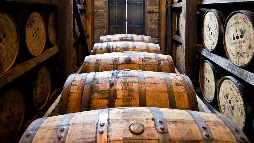
In 1933, a precedent was set for paying whisky as a dividend on common stock. As I have discussed in an earlier blog, entitled The Famous Whiskey Dividend, companies can invent creative ways to pay out dividends. In fact, when the going gets tough, the tough go drinking. After Prohibition was repealed in 1933, National Distillers Products Corporation distributed a dividend of one case of whiskey for each five shares that were owned. This pulled out the stops with paying dividends. Twenty years later, Park & Tilford provided a more sobering saga.  

PUMP AND DUMP

Originally founded in 1840, Park & Tilford had a long history of being a family-owned operation run by the Schulte’s. For decades, the company produced a broad line of whiskey and related products until it formally incorporated in 1923 in order to list on the NYSE. In 1943, in the middle of World War II, whiskey was scarce. Most companies that produced whiskey had their factories diverted to manufacturing more important goods – in the opinion of some folks – making whisky a hot product to the public. Since Park & Tilford owned a drug store in New York and went public during prohibition; the company diversified into cosmetics, perfumes and other drug sundries. Though Prohibition had been repealed in 1933, the diversion of resources to the production of war materiel had some people worried that Prohibition was being reintroduced de facto if not de jure. On December 15, 1943, D.A. Schulte, the President of Park & Tilford announced that the company was contemplating a distribution of whiskey to its shareholders. The announcement by Schulte had its effect. Based on these rumors, the stock advanced roughly 40 points over the next five months, as new shareholders tried to get access to scarce whisky to sell on the black market. This advance was an aggressive move in any market. The Schulte family owned over 90% of Park & Tilford stock, and they took advantage of the promise of the whiskey dividend to sell their stock to the public During the five months that followed the announcement, the family unloaded 93,000 shares through their broker, Ira Haupt & Co. The 93,000 shares the family sold may not seem like a large amount of stock until you realize that there were only 243,683 shares outstanding when the whiskey announcement was made. Ira Haupt & Co unloaded 40% of the outstanding shares as the stock hit new highs between December 1943 and May of 1944, as can be seen by the graph below. Park & Tilford stock had been at 57.625 on December 15, 1943 and advanced to 98.25 on May 26, 1944. It was classic pump and dump. Pump up the stock price then dump the shares on unwitting investors.

WHISKY DIVIDENDS

On May 26, the company formally announced the details of the whisky dividend. During World War II, the government imposed price controls on consumer goods, including liquor. The Government did not see the whiskey dividend as an exception to their regulations. The Office of Price Administration stepped in and limited the negotiability of the purchase rights and the maximum profit on the resale of the liquor. The stock price plummeted on the news. Since some shareholders were more interested in making cash than in drinking whiskey, they saw their profits from the whiskey dividend melt away, further causing a collapse in the stock price. If the government had not intervened with their ruling, the result might have been otherwise, but the government did intervene. The price of Park & Tilford fell 10 points on May 31st; and declined over 60 points during the month of June to close at 32 on June 28. The stock’s behavior relative to the S&P 500 is shown in the graph below.

LIQUID STOCKS

Until the announcement, Park & Tilford stock had been relatively illiquid. In the month of November 1943, only 7,000 shares of Park & Tilford had traded on the NYSE, but after the announcement was made, 24,500 shares, or about 10% of the float, traded in the next two days, and 115,000 shares, or half the float, traded during the rest of the month. The announcement of the whiskey dividend had made their stock very liquid. Unloading such a large number of shares caused Park & Tilford and the brokerage firm of Ira Haupt & Co. to run afoul of the SEC. During the period in which the 93,000 shares were dumped on the public, ten representatives of Ira Haupt & Co. solicited twenty-one customers to buy shares in the company, and the company’s chief statistician prepared a written analysis of the stock for a customer. The sale of stock by the Schulte family was, essentially, a secondary offering since the company had used a brokerage firm to distribute the stock. In a secondary offering, potential buyers know that insiders in the firm are unloading stock and the float is increasing. This tends to drive down the price of the stock. Park & Tilford used the rumors they had circulated about the Great Whiskey Dividend to push the price up so the family could unload their shares at a higher price; however, potential buyers were completely unaware they were buying shares from insiders.  

A TOAST TO PUMP AND DUMP

Though Park & Tilford argued that the shares they sold were not a secondary offering, the SEC saw otherwise and ruled against Park & Tilford and Ira Haupt & Co. since “[t]he only reasonable conclusion that could have been reached by respondent was that it was intended that a large block would be sold.” This rule was formalized by the SEC in Rule 154 which was adopted in 1954. If Park & Tilford’s principal shareholders had only sold a few hundred shares, there would have been no violation of SEC rules, but since the company had unloaded a large block of shares, they were effectively making a secondary offering. Ira Haupt & Co. should have insisted on a registration statement for the securities being distributed from Park & Tilford, and should have provided potential customers with a prospectus, but they did not. As a result, Ira Haupt & Co.’s membership in the NASD was suspended for twenty days. What have we learned here? Besides the fact that investors need to have all of the facts before investing, they also need to have a brokerage firm that is transparent with all relevant information, just the opposite of the behavior of Ira Haupt & Co. Had investors known they were being solicited to buy shares from insiders, and that the government was going to limit the profitability of the Whisky Dividend, the stock would never have risen in price as it did in order to be dumped by the Schultes. This is a classic case of not only buy on rumor and sell on news and don’t count your chickens before they are hatched, but most importantly, there is a sucker born every minute.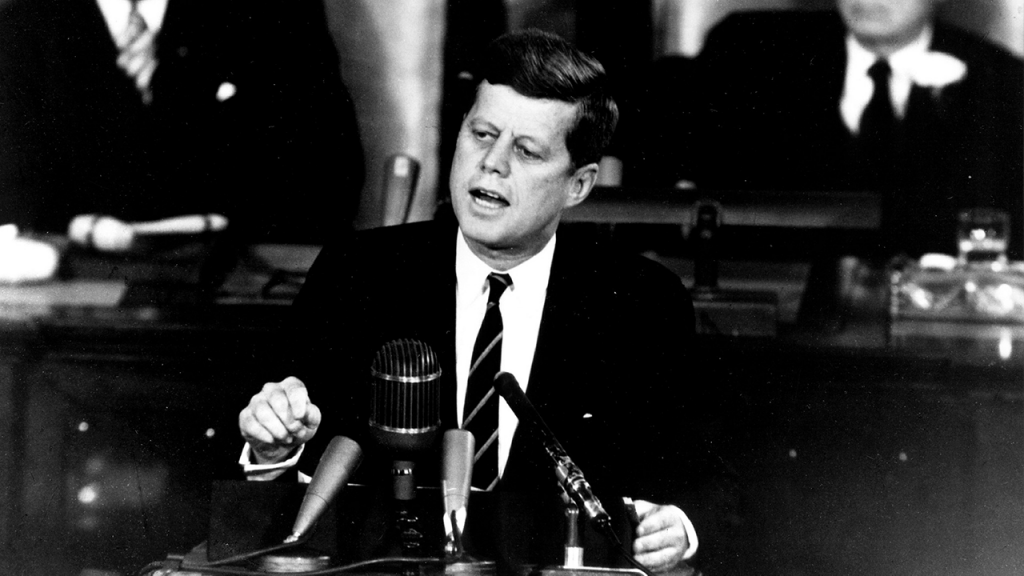

  Fifty years ago, John F. Kennedy was assassinated on Friday, November 22, 1963 in Dallas, Texas. The assassination not only shocked the nation, but shook the stock market as well. However, very few people have heard about The Great Salad Oil Swindle which nearly crippled the New York Stock Exchange that weekend. Officials at the NYSE took advantage of the closure of the exchange to keep the crisis caused by the swindle from spreading further. Here is what happened at the NYSE while the nation focused on the President’s funeral.

Salad Oil, Cornered and Quartered

The Great Salad Oil Swindle was carried out by Anthony “Tino” De Angelis, who traded vegetable oil (soybean oil) futures which was an important ingredient in salad oil. De Angelis had previously been involved in a swindle involving the National School Lunch Act while he President of the Adolph Gobel Co. When it was discovered that he had overcharged the government and delivered over 2 million pounds of uninspected meat, he and the company ended up bankrupt. Con-men don’t stop being cons, they just try to learn from their mistakes and make more money the next time around. Buying soybean oil futures would drive up the price of his vegetable oil holdings, which would increase both the value of his inventories and allow him to profit from his futures contracts. De Angelis could use these profits not only to line his own pockets, but to pay his staff, make contributions to the community, and in one case, pay the hospital bill of a government official. American Express had recently created a new division that specialized in field warehousing, which made loans to businesses using inventories as collateral. American Express wrote De Angelis warehouse receipts for millions of pounds of vegetable oil, which he took to a broker and discounted the receipts for cash. This proved to be an easy way to get money, so De Angelis began falsifying warehouse receipts for vegetable oil he didn’t have. American Express sent out inspectors to make sure that De Angelis had the vegetable oil that acted as collateral, but what they didn’t know is that many of the tanks were filled mostly with water with a minimum of oil floating on the top to fool the inspectors, or that some of the tanks were connected with pipes to other tanks so the oil could be transferred between tanks when the inspectors went from one tank to the other. If American Express had done their homework, they would have realized that De Angelis’s reported vegetable oil “holdings” were greater than the inventories of the entire United States as reported by the Department of Agriculture. Unsatisfied with the American Express loans, De Angelis was able to get additional loans from Bunge Ltd., Staley, Proctor and Gamble, and The Bank of America. By the time the swindle collapsed, De Angelis had gotten loans from a total of 51 companies.  

No Salad Today

When De Angelis got a large order from Spain, he started speculating in the futures market to increase his profits, but when the order was reversed, he decided to prop up the market rather than cut his losses. De Angelis pulled out all the stops. He forged warehouse certificates, stole warehouse certificates, kited checks and warehouse certificates, opened a new brokerage account at Ira Haupt & Co., and even attempted to bribe employees of other companies. You can’t hold up the market forever. Eventually, the whole house of cards collapsed. Inspectors were eventually tipped off about De Angelis’s fraud. Allied Crude was supposed to have $150 million in vegetable oil as collateral, but only had $6 million. When the inspectors found water in the tanks, and not oil, the gig was up. The futures market crashed. Soybean oil closed at $9.875 on Friday, November 15, at $9 on Monday and $7.75 on Tuesday, November 19, wiping out the entire value of the De Angelis loans. As you might guess, De Angelis’s company had been losing money all along, and the loans were used to cover these mounting losses. De Angelis’s goal was to sell out at the top and cover all of his losses, but of course, his plan didn’t work out that way. The crash of the soybean oil market in November 1963 is shown below. On Friday, November 22, the NYSE organized a bail out of Williston & Beane, and the firm was allowed to reopen at noon on Friday. Ira Haupt & Co. was a bigger problem. It collectively owned $450 million in securities and owed various banks over $37 million that it could not pay. At 1:41 pm, as soon as word that JFK had been shot flashed on the floor of the New York Stock Exchange (NYSE), began to sell off. The Dow Jones Industrials, which was recorded at hourly intervals in 1963, had been at 735.87 at 1 pm on November 22, ultimately declined to 730.18 by 2 pm. Over the next seven minutes, the market traded 2.2 million shares and lost an additional nineteen points, erasing around $11 billion in capitalization, before NYSE officials halted trading at 2:07 pm to stop the panic selling. The market rested, and the next day, JFK’s body lay in repose at the White House. On Sunday JFK’s was taken to the rotunda of the Capitol for public viewing. Over 250,000 people viewed the casket as a line stretched for 40 blocks, or 10 miles. Some people waited over 10 hours in the freezing cold to pay their last respects. On Monday, the casket was transferred to the National Cathedral where his funeral mass was broadcast to a stunned nation. Kennedy was buried in Arlington Cemetery, where the eternal flame was lit over his grave. The stock market remained closed on Monday and reopened on Tuesday, November 26, when the market traded over 9 million shares, closing the day at 743.52, moving up 4.5% from the previous day’s close. The table below provides the hourly performance of the DJIA on November 22 and 26, 1963

In the past, anyone could invest in fledgling companies before they listed on the NYSE. Today, this opportunity is rarely available to the average investor. This is illustrated by the outperformance of other companies, such as Xerox, Dr. Pepper and Kentucky Fried Chicken. By the time these companies moved onto the NYSE, a good portion of the advance in their stock price had already occurred. If you ignore the performance of the stock when it traded over-the-counter, you miss a substantial portion of the stock’s historic move, and without this information, you will never fully understand the returns that were available to investors in the past.  

Disney Trades on the OTC in 1946

Walt Disney Productions incorporated in 1938. The company issued its 6% Cumulative Convertible Preferred to the public in 1940; its common began trading OTC in 1946; and the company listed on the NYSE on November 12, 1957. If you study the changes Walt Disney made to his eponymous company before it listed on the NYSE, you can see how he primed the company to increase in price and make sure the listing on the NYSE was successful. Walt Disney, his brother Raymond and their wives owned over 25% of the stock. These shares were later put into the Disney Family Voting Trust which held 46.8% of the common stock in 1959. Having such a large ownership of the shares, Walt Disney had every incentive to drive the price up. The Preferred stock was issued at $25, but the company suffered large losses in 1941, caused by the disappointing returns from Pinocchio and Fantasia which were not as successful as Snow White had been. The company failed to meet its preferred dividend in July 1941. The company fell in arrears on the dividend, but since the preferred was cumulative, there was always the chance the company would make up the lost dividends, and they did. Disney restarted the regular dividend in July 1947, and caught up on the $7.50 in arrears in 1948 and in 1949. You can see the impact of this on the preferred stock, which had fallen in price to $3.50 by April 1942, rising to $32.50 by the beginning of 1946 to reflect the expectation of the missed dividends being paid. This is also when the company’s common began trading OTC. The preferred stock, whose chart is provided below, was redeemed on January 1, 1951 at $25 with all dividends paid.

Transforming Tomorrowland before Neverland

In the twelve years between 1946, when Disney common started trading OTC, and when it listed on the NYSE on November 12, 1957, Walt Disney introduced numerous innovations that transformed the company and increased its profits. Disney made animated films that had been delayed by the war, such as Alice in Wonderland, Peter Pan and Cinderella. The company began making live action movies with Treasure Island in 1950 and 20,000 Leagues under the Sea in Cinemascope in 1954. For TV, Disney introduced the Disneyland TV show (later Walt Disney’s Wonderful World of Color) in 1954, and the Mickey Mouse Club began production in 1955. Of course, Walt’s greatest innovation was Disneyland, which opened on July 17, 1955 for which Walt Disney hosted a live TV preview with Ronald Reagan and others. Note that all of these events occurred before Walt Disney Productions, as it was known then, listed on the NYSE. In the year before the stock first traded on the NYSE, the company did a 2-for-1 stock split and paid its first dividend on the common stock. One difference between Disney in the 1950s and Facebook or Twitter in the 2010s is that anyone could have bought the stock OTC before it listed on the NYSE. The stock wasn’t restricted to employees and venture capitalists. Anyone who went to Disneyland in 1955, watched the Mickey Mouse Club or the Disneyland TV show, or saw the movies Disney was releasing could have taken advantage of the company’s growth. The chart below shows how Disney stock performed between 1946 until 1975. The stock traded at 3 in 1949, moved up to 52 by July 1956 before splitting 2-for-1. The stock closed at $13.75 on November 12, 1957 when it debuted on the NYSE, and moved up to $59.50 by April 1959. The stock traded sideways until 1966 when it began another significant move as one of the “Nifty Fifty” stocks of the 1960s, hitting 244 by the beginning of 1973. One important difference between Disney and Facebook or Twitter was in the accessibility of the stock. Disney’s 6% Preferred was available OTC from 1940 to 1950 during which an investor could have made a 10-fold profit. The common stock made a 10-fold move between 1949 and its debut on the NYSE in 1957, then another 10-fold move by 1973 while it was a member of the Nifty Fifty in the 1960s. Since 1973, Disney stock has moved up another 30-fold. On a total return basis, even ignoring the 10-fold move in the Disney 6% Preferred, $1 invested in Walt Disney Productions common in 1948 would be worth over $48,000 today, assuming all dividends had been reinvested. Even $1 invested in Disney on November 12, 1957 would be worth $5,000 today. Disney certainly has been one of the top performing stocks on the NYSE since it debuted there in 1957; however, once you take into consideration the profits an investor could have made if they had bought Disney Preferred OTC in 1941, and had switched to the Common Stock when the Preferred was called, the returns increase 100-fold. Based upon Disney’s returns OTC and on the NYSE, Disney probably has the “happiest” shareholders on Earth.

The foundations of the VOC were laid when the Dutch began to challenge the Portuguese monopoly in East Asia in the 1590s. These ventures were quite successful. Some ships returned a 400% profit, and investors wanted more. Before the establishment of the VOC in 1602, individual ships were funded by merchants as limited partnerships that ceased to exist when the ships returned. Merchants would invest in several ships at a time so that if one failed to return, they weren’t wiped out. The establishment of the VOC allowed hundreds of ships to be funded simultaneously by hundreds of investors to minimize risk. 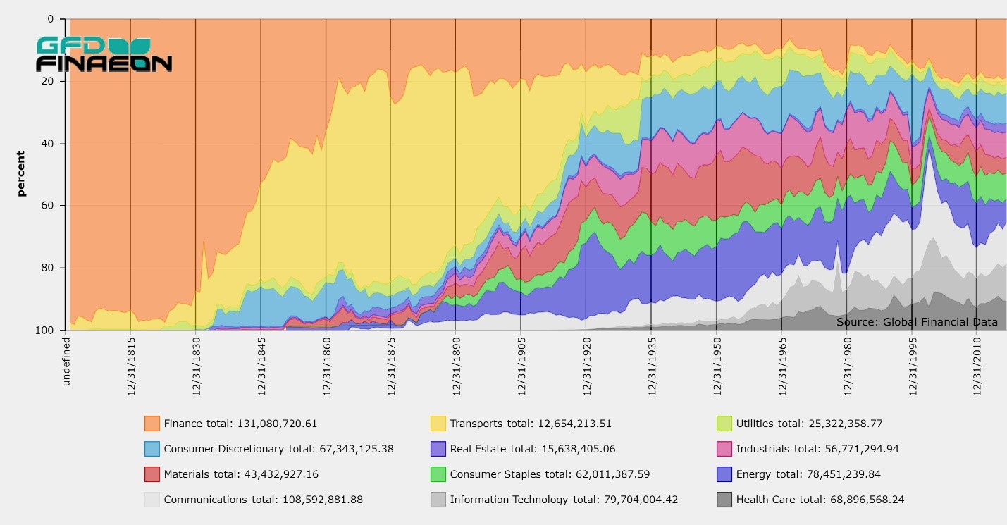The English founded the East India Company in 1600, and the Dutch followed in 1602 by founding the Vereenigde Oost-Indische Compagnie. The charter of the new company empowered it to build forts, maintain armies, and conclude treaties with Asian rulers. The VOC was the original military-industrial complex. The VOC quickly spread throughout Asia. Not only did the VOC establish itself in Jakarta and the rest of the Dutch East Indies (now Indonesia), but it established itself near Japan, being the only foreign company allowed to trade there, along the Malabar Cost in India, removing the Portuguese, in Sri Lanka, at the Cape of Good Hope in South Africa, and throughout Asia. The company was highly successful until the 1670s when the VOC lost their post in Taiwan, and faced more competition from the English and other colonial powers. Profits continued, but the VOC had to switch to traded goods with lower margins, but they were able to do this because interest rates had fallen during the 1600s. Lower interest rates enabled the VOC to finance more trade through debt. The company paid high dividends, sometimes funded by borrowing, which reduced the amount of capital reinvested. Given the high level of overhead it took to maintain the VOC outposts throughout Asia, the borrowing and lack of capital ultimately undermined the VOC. Nevertheless, until the 1780s, the VOC remained a huge multinational corporation that stretched throughout Asia. The Fourth Anglo-Dutch War of 1780-1784 left the company a financial wreck. The French Revolution began in 1789, leading to the occupation of Amsterdam in 1795. The VOC was nationalized on March 1, 1796 by the new Batavian Republic, and its charter was allowed to expire on December 31, 1799. Most of the VOC’s Asian possessions were ceded to the British after the Napoleonic Wars were finished, and the English East India Company took over the VOC’s infrastructure. The VOC transformed financial capitalism forever in ways few people understand. Although shares had been issued in corporations before the VOC was founded, the VOC introduced limited liability for its shareholders which enabled the firm to fund large scale operations. Limited liability was needed since the collapse of the company would have destroyed even the largest investor in the company, much less the smaller investors. Although this innovation changed capitalism forever, there were ways in which the VOC failed to transform itself, which led to its downfall. The company’s capital remained virtually the same during its 200 year existence, staying around 6.4 million florins (about $2.3 million). Instead of issuing new shares to raise additional capital, the company relied on reinvested capital. The VOC’s dividend policy left little capital for reinvestment, so the company turned to debt. The company first issued debt in the 1630s, increasing its debt/equity ratio to two. The ratio stayed at two until the 1730s, rising to around four in the 1760s, then increased dramatically in the 1780s to around 18, ultimately bankrupting the company, and leading to its nationalization and demise. In the 1600s and 1700s, the Dutch had the lowest cost of capital in the world. This was because of an innovative idea: if you pay back your loans, your creditors will reward you with a lower interest rate. This wasn’t the way Spain, France, and other kings looked at borrowing money, and their interest rates remained high. As a result of Dutch fiscal rectitude, the yield on Dutch government bonds fell from 20% in 1517 to 8.5% by 1600 and to 4% by 1700. Not only did the Dutch have the lowest interest rates in the world at that time, but they had the lowest interest rates in history. This pushed the Dutch to invest not only in joint-stock companies, such as the VOC, but in foreign government debt, helping to fund the American Revolution. Another interesting aspect of the VOC was its dividend policy. Some of the dividends were paid in kind, rather than in money, and the dividends varied widely. The company paid dividends of 15% of capital in 1605, 75% in 1606, 40% in 1607, 20% in 1608, 25% in 1609 in money, then an average of 71% in produce for the next seven years, the next 5 years in money at 19%, the next three years in cloves at 41%, 44% in spices in 1638, in 1640 two dividends of 20% each, 5% in money and 15% in cloves, 1641, 40% in cloves, 1642, 50% in money, 1643, 15% in cloves, from 1644 to 1672, an average of 21.25% per annum, all but one paid in money, in 1673, bonds for 33.5% were given, payable by the province of Holland, from 1676 to 1682, 4% bonds averaging 19.5% of par per year, from 1683 to 1689, money averaging 20%, from 1690 to 1698, bonds paying 3.5% payable in 1740 on average of 21.875% per annum, from 1698 to 1728, money was paid, averaging 28.125% per annum. The dividend averaged around 18% of capital over the course of the company’s 200-year existence, but no dividends were paid after 1782. The VOC provided a high return to investors, but not always in the way shareholders wanted. The VOC basically unloaded their inventories on shareholders in some years, providing them with produce, cloves, spices or bonds. Some shareholders refused to accept them. Obviously, shareholders want money, not goods, and the three British companies, Bank of England, East India Company and South Sea Company, learned from this and only paid cash dividends during the 1700s. The average dividends of 20-30% of capital were high, but since the price of shares traded around 400 during most of the company’s existence, as the chart below shows, the actual dividend yield was around 5-7%, better than Dutch bonds, but less than bonds from “emerging market” countries, such as Russia or Sweden. The VOC also transformed the Amsterdam Stock Exchange, causing a number of innovations to be introduced, such as futures contracts, options, short selling, and even the first bear raid. Isaac le Maire was the largest shareholder of the VOC in its early years, and he initiated the first bear raid in stock history, selling shares of VOC short in order to buy them back at a profit and buy additional shares. These actions also led to the first government regulation of stock markets, attempting to ban short selling in 1621, 1623, 1624, 1630 and 1632 as well as options and other forms of financial wizardry. The fact that these laws had to be passed so many times shows the regulations were not that effective. One problem for the long-term success of the Amsterdam Stock Exchange was that the VOC and the West Indies Company (WIC) were the only shares of importance that traded on the Amsterdam Stock Exchange. Between 1600 and 1800, no new large companies listed in Amsterdam. Although Dutch fiscal rectitude kept debt and interest rates low, it also helped stifle the growth of the Amsterdam Stock Exchange because government bonds never became a prominent part of the trading on the exchange. Due to the decentralized political nature of the Netherlands, government debt was held locally. There was no centralized national debt as in France and England, and ultimately, this inhibited the growth of the Amsterdam Stock Exchange. The Netherlands was as decentralized as France was centralized. Because the VOC and WIC so dominated the share market, the company didn’t issue new shares to raise capital, and Dutch debt was so small and diversified among its cities, that the Dutch invested in foreign debt to find an outlet for their capital. Dutch newspapers of the 1700s often list the prices of French debt in Paris as well as British Consols, Bank of England Stock, British East India Company and South Sea Company stock in London, but no other debt or equity from Amsterdam is listed. With the exception of colonial trade, until the 1800s no capitalist enterprise required the levels of capital of the VOC and WIC. So the Dutch capital that was available went into debt, not equity. America went to Amsterdam to raise capital, as did Sweden, France, England, Russia, Saxony, Denmark, Austria and other countries. This provided Dutch investors with higher returns, but didn’t develop the Dutch economy in the way it could have. Another factor that may have held the Amsterdam Exchange from expanding was the fact that shares could only be registered on a monthly or quarterly basis. The situation was different in London. Not only could British shares and debt be registered daily, but all of the shares were available for transfer. On the other hand, many VOC shares weren’t traded at all. The amount of British and French debt grew throughout the 1600s and 1700s, requiring new investors on a regular basis. Not only did the VOC’s capital remain constant, but centralized Dutch government debt didn’t exist until the Netherlands became a kingdom under Napoleon. Amsterdam failed to provide its investors new opportunities. Before the Industrial Revolution, companies were simply too small to require sufficient capital to be traded on exchanges. Shipping had long been a high-risk venture, providing high returns and high losses, and investors diversified their risk by putting their money in a number of different ships. The colonial trading companies of the 1600s and 1700s took financial capital to a different level, allowing thousands of people to invest in thousands of shipping ventures and diversifying risk. After the Napoleonic Wars, the center of global finance shifted from Amsterdam to London. Although this process was spread out over several decades, it is amazing that the center of global finance could so easily switch from Amsterdam to London so quickly and easily. There were some things, mostly political, which Amsterdam had little control over, such as the Napoleonic Wars, their occupation by the French, and the loss of its colonies after the war. In retrospect, there were things the Dutch could have done to increase the likelihood that Amsterdam would have stayed at the center of global finance after 1815, though they probably could not have foreseen that the center would shift to London. The Dutch failed to diversify away from VOC and WIC shares and allow other companies to take advantage of capital markets; they failed to sufficiently develop the bond side of the market because was no centralized government debt; they failed to expand the capital of the VOC, but instead chose to borrow, adding to the debt load which led to the bankruptcy of the VOC and WIC; the VOC and WIC did not sufficiently reinvest dividends for growth, and they failed to offer a large number of securities that would encourage trading as in London. The company failed to raise additional capital when necessary, to limit borrowing, or to fund capital expenditures through cutting its dividend. Since the Netherlands lacked a centralized debt issuer, as the French, British and Russians did, the Amsterdam Stock Exchange faded in importance after the VOC and WIC collapsed. Foreign government bonds became more prominent in Amsterdam, but even the foreign government bond trading moved to London in the 1820s where capital was more readily available. It is doubtful whether Amsterdam could have foreseen all the changes that happened, and perhaps they couldn’t have prevented the switch from Amsterdam to London that occurred after 1815, but it was a lesson London should have learned. London became the engine of global capitalism for the nineteenth century, only to lose its place to New York after World War I. The US should understand this lesson as well. The global center of finance must grow, innovate and be as open as possible. Otherwise, the center will move to someplace that is.