Global Financial Data has the most extensive database on historical stocks available anywhere in the world. GFD has collected data on stocks that listed on the London Stock Exchange from the 1600s until 2018. London was the financial center of the world until World War I, and many companies in emerging markets listed their shares on the London Stock Exchange before a stock exchange even existed in their country. After World War I, many foreign companies listed on the New York Stock Exchange. Using data from London and New York, we can calculate stock market indices for emerging markets during the 1800s and 1900s before stocks listed on local exchanges and local emerging market indices were calculated. This is one in a series of articles about those countries.
The Suez Canal Connects the World
There were a number of companies that listed in London and Paris as well as on the Cairo and Alexandria Stock Exchanges in the 1800s and 1900s. The first company for which GFD has data is the Bank of Egypt which traded in London from 1856 until 1910. Several other companies came along in the 1860s including the Egyptian Commercial and Trading Co. (1863), Societe Financiere d’Egypt (1864) and the Anglo-Egyptian Banking Co. (1865-1920). However, the largest company in Egypt, the Compagnie universelle du canal maritime de Suez (Suez Canal Co.) went public in 1858 and ran the Suez Canal until it was nationalized by Egyptian President Gamal Abdel Nasser in 1956. GFD has data on the Suez Canal from its IPO in 1862 until 1940. During the late 1800s, the Suez Canal Co. was one of the largest stocks by capitalization that traded on either the Paris or the London Stock Exchange.
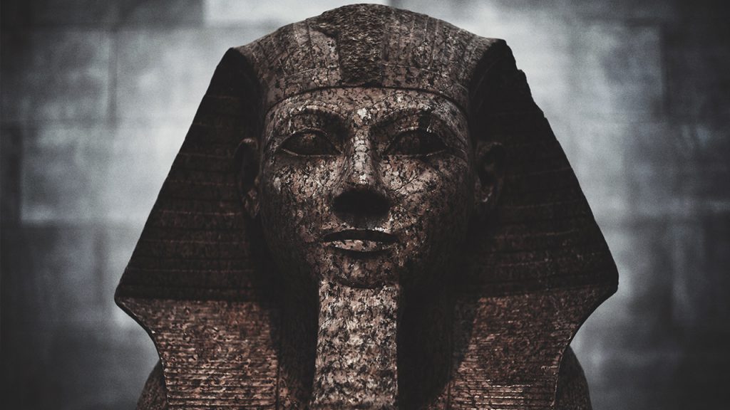
The Suez Canal was constructed between 1859 and 1869 and was officially opened on November 17, 1869. Dreams of building a canal between the Mediterranean and the Red Sea go back almost 4000 years, but until the 1800s, no one had succeeded in building a useable canal. In 1856, Ferdinand Lesseps obtained a concession from Sa’id Pasha, the Khedive of Egypt and Sudan to create a company that would construct a canal open to ships from every nation. The Suez Canal Co. was founded on December 15, 1858 with the Egyptian government owning 44% of the shares, and French and Egyptian investors owning the rest. The company issued 400,000 shares at 500 francs ($100) each, giving the company a market cap of $40 million.
Work on the canal began on April 25, 1859. Both the transcontinental railroad in the United States and the Suez Canal were opened in 1869 making it easier to conduct trade around the world. Sa’id Pasha defaulted on government bonds in 1875, and he sold his 44% stake in the Suez Canal Co. to Britain which became the largest shareholders in the canal. The British invaded Egypt in 1882 to suppress the Urabi Revolt and in 1888, the Convention of Constantinople declared the canal a neutral zone under the protection of the British. The canal was nationalized in 1956 and shareholders were paid off by 1962, though hardly at a rate that was in their favor.
As Kindleberger put it, “Said and Ismail were profligate viceroys, borrowing in Europe at high interest rates for consumption, for irrigation schemes designed to serve their own estates, for an extravagant fête to celebrate the opening of the Suez Canal, for badly planned public works. The railroads and Suez Canal benefitted Europe, for example not Egypt, and cost Egypt £12 million for shares ultimately sold to the British government under Disraeli for £4 million. In all, the Egyptian government under Ismail (after 1863) borrowed £53 million, received only £32 million, paid £35 million in debt service, but still owed £52 million on capital account and arrears of interest in 1876 when the government finally defaulted. Marlowe (a nom de plume) observes that it was easy to castigate the Europeans who made every Ismail initiative contribute to their wealth, but Egyptian mismanagement was itself spectacular.” (Charles Kindleberger, A Financial history of Western Europe, London: George Allen & Unwin, 1984, p. 224)
Figure 2 below shows the performance of Suez shares between 1862 and 1940. As can be seen, shares in the Suez Canal rose in price from 1858 until World War I, declined in price until the early 1920s, then made a dramatic rise until 1939 when World War II caused the price of Suez Canal Co. shares to crash back to the level of the 1920s.
Egyptian Stock Market Returns
When Suez shares started trading in London in 1875, the Suez Canal Co. represented 75% of the market cap of all Egyptian shares listed in London, and in 1940 when shares stopped trading, the Suez Canal Co. still represented about 85% of the market capitalization of Egyptian shares that traded in London. Therefore, GFD’s Egyptian stock index is more an index of shares in the Suez Canal than an index of shares in Egyptian stocks. For this reason, we have calculated GFD’s index of Egyptian stocks both with and without Suez shares so the two can be compared. Generally speaking, the Suez Canal Co. was also one of the largest companies traded in Paris with only the Paris, Lyons and Mediterranean Railway and Northern of France Railway being larger at the end of the 1800s. By 1900, the Suez Canal Co. was the largest company listed on the Paris Stock Exchange.
Most of the other companies that were listed in London were either banks or real estate companies. This included the National Bank of Egypt (1899-1958), which was nationalized in 1960, the Bank of Egypt (1856-1910), the Land Bank of Egypt (1907-1930) and the Agricultural Bank of Egypt (1904-1837). Other prominent companies included the Egyptian Salt and Soda Co. (1905-1930), Anglo-Egyptian Oilfields Ltd. (1910-1961), Land and Mortgage Co. of Egypt (1880-1926), Alexandria Water Co. (1905-1930), Egyptian Markets Ltd. (1906-1927), and the Egyptian Delta Land and Investment Co. (1909-1930).
The Alexandria Stock Exchange was founded in 1883 and the Cairo Stock Exchange in 1903. The market cap of Egyptian shares that traded in London remained quite high, primarily because of the Suez Canal Co. In 1937, the market cap of Egyptian shares exceeded $1 billion, although only about $100 million of this was from non-Suez Companies. Figure 3 shows the performance of all Egyptian shares listed in London from 1856 until 1969. The index peaked in 1929 and had lower highs in 1937, 1945 and 1955 right before the Suez crisis.
Between 1856 and 1969, Egyptian stocks increased in price at an annual rate of 2.31% and 7.55% on a return basis, giving a dividend yield of 5.12%. But this obscures the huge variance in returns over time. Between 1856 and 1912, Egyptian stocks rose at an annual rate of 6.83% and by 5.82% between 1846 and 1929. Add on another 5% for dividends Egyptian stocks provided good returns during its heyday, though primarily because of the strong performance of Suez Co. shares.
What does the Egyptian stock market look like if Suez is excluded from the index? To find this out, we calculated an Egypt x/Suez index which is reproduced below. Figure 4 shows peaks at similar times as the graph above, with the market topping out in 1929, 1937, 1945 and 1955, but the total return is completely different with the index increasing only 0.14% per annum from 1856 to 1961 and 6.37% with dividends reinvested. Between 1856 and 1929, the annual increase in the price of Egyptian stocks was only 2.00% per annum versus 5.82% once Suez stock is included. In other words, without Suez stock, Egyptian shares behaved just like shares from any other country, fluctuating up and down, but providing little if no long-run return to shareholders. All the return came through dividends.
Egypt did calculate a stock market index of shares that listed in Cairo and Alexandria between 1948 and 1962 when Nassar nationalized a number of Egypt’s companies which is illustrated in Figure 5. Share trading declined after 1962 and no index is available for Egypt until 1980.
The Future of Egypt
Egypt is a unique emerging market because of the dominance of the Suez Canal Co. in the Egypt’s market cap. The Suez Canal Co. was a French company with operations in Egypt with the British owning the largest number of outstanding shares. The Suez Canal Co. played such a prominent role in Paris that David le Blis included it as one of the stocks in their index of 40 shares that traded in Paris between 1852 and 1987. The Suez Canal Co. consistently represented over 75% of the market cap of the Egyptian stock market. When the Egyptian government nationalized the canal in 1956 and paid it off in 1962, there were few Egyptian shares left for investors to trade in either Egypt or London.
Nevertheless, during most of its history, the Suez Canal Co. provided a liquid market which generated decent returns to its shareholders. However, Egypt is still struggling politically to provide the economic foundations that will enable the country to emerge as a developed economy. Whether Egypt can overcome its political problems and become a more market-oriented economy that follows in the footsteps of Israel and creates companies that can make products that investors prize throughout the world remains to be seen.


 Most global markets are in a bear market. The main question everyone is asking is whether the bear market will continue in 2019 and hit new lows, or whether the stock market will find a bottom and start to move up again. Last year, we were optimistic that markets were in a bull market, but our hopes were quickly dashed. Many European markets hit market tops at the end of January, and the rest of the world slid into a bear market after Labor Day. It was hoped that the September-October decline would turn around at the end of the year, but December was the worst December in the United States since 1931 as the United States slid into a bear market.
The United States and the MSCI World Index had avoided a bear market in 2016 when the rest of the developed world faced 20% declines, but this time, the United States was not so lucky. The MSCI World Index and the EAFE Index, illustrated in Figure 1, topped out on January 26, and the S&P 500 topped out on September 21. As the graph illustrates, the EAFE Index is at the same level it reached in 1999. The main question is how long will this bear market last? The bear market in 2000 lasted almost three years while the 2007-2008 bear market lasted a little over a year. We have been in the current bear market for almost a year. Is worse to come in 2019?
Most global markets are in a bear market. The main question everyone is asking is whether the bear market will continue in 2019 and hit new lows, or whether the stock market will find a bottom and start to move up again. Last year, we were optimistic that markets were in a bull market, but our hopes were quickly dashed. Many European markets hit market tops at the end of January, and the rest of the world slid into a bear market after Labor Day. It was hoped that the September-October decline would turn around at the end of the year, but December was the worst December in the United States since 1931 as the United States slid into a bear market.
The United States and the MSCI World Index had avoided a bear market in 2016 when the rest of the developed world faced 20% declines, but this time, the United States was not so lucky. The MSCI World Index and the EAFE Index, illustrated in Figure 1, topped out on January 26, and the S&P 500 topped out on September 21. As the graph illustrates, the EAFE Index is at the same level it reached in 1999. The main question is how long will this bear market last? The bear market in 2000 lasted almost three years while the 2007-2008 bear market lasted a little over a year. We have been in the current bear market for almost a year. Is worse to come in 2019?