GFD is revising its stock index for Australia because it can now use data on Australian shares that were listed in London to supplement the data that already exists from Sydney and other Australian exchanges. Australia has one of the highest returns of any stock market in the world, but this is in part due to problems with the indices that were calculated in the 1950s and the biases in that data. Historical data for Australia was calculated by Lamberton in the 1950s, but the data are limited to commercial companies and ignores returns to mining and finance companies. A similar problem exists with the indices calculated by Schumann and Scheurkogel for South Africa. Once you add in the returns to finance and mining companies, Australian returns decline to a more realistic level.
The Lamberton Australian Stock Exchange Indices
When Lamberton completed his calculation of returns in 1957, he lacked the computers that were needed to create market-cap weighted indices that are now recognized as the standard for stock market index calculations. Consequently, he used short cuts that created biases in his indices. First, the price indices were unweighted giving small companies the same weight as large companies. Second, the dividend data were unweighted measures of the yield on all shares. Third, the data that were used were monthly averages rather than end-of-the-month values. Fourth, there was rapid turnover in the stocks which were few in number. In 1880, the index included just five members, and of the 40 members in 1920, just 11 remained in 1925. These four factors bias the results of the Lamberton indices. Lamberton’s biases have crept into the data in two other ways. First, most people have used the returns to commercial/industrial stocks to calculate the returns to Australian stocks and have ignored mining and finance stocks. The commercial/industrial shares had excessively high returns that exceeded the returns on finance and mining shares. Second, the calculation of dividends was equal-weighted rather than market-cap weighted. It has been estimated that Lamberton’s methodology added at least two percentage points to the actual dividend yields on Australian stocks. According to Lamberton’s calculations, the average dividend yield was 6.77% between 1882 and 1957, which is about 2 percentage points higher than the 4.45% dividend yield that was paid to British shares in London between 1882 and 1957. Lamberton also calculated three indices for stocks in Australia: mining, finance and commercial/industrial shares. The mining share index was calculated from 1875 until 1910, and during that time, mining stocks declined in price by 0.80% per annum. During the same period of time, finance stocks increased 1.57% per annum while commercial/industrial shares increased by 3.56% per annum. If you cover the full period from 1875 to 1955, annual returns on the commercial/industrial shares was 4.08% and the return on the finance shares was 1.01%. If you add the 6.77% dividend yield on commercial shares from 1882 to 1957, you get an annual return over 10% for 80 years during a period when shares in London returned 5.92% on average. Since many Australian shares traded in London, it seems hard to believe that a 4% difference in the rate of return to Australian and British shares could persist for 75 years. Why would someone invest in non-Australian shares if they knew they were going to get a 4% lower return each year? On the other hand, “real time” data exists for Australian indices between 1958 and 2018. During that period of time, share prices in Australia rose 6.23% per annum and 11.83% after dividends while inflation rose 4.67%. This gives an annual real total return of about 7% after inflation between 1958 and 2018. This is much lower than the Australian data from 1882 to 1958 and comparable to returns in the United States and other countries. By calculating indices for mining and finance shares that were listed in London, we can make direct comparisons between Lamberton’s equal-weighted results and GFD’s returns to test the validity of Lamberton’s results. To use one example, between 1887 and 1888, Lamberton’s mining index tripled in price, then lost half of its value, but GFD’s Materials index hardly budged during the same period that Lamberton’s index tripled. When we looked at the actual data, we found that over one-third of the total market cap in the GFD index came from Day Dawn Block & Wyndham Gold Mining Co. Ltd. which declined in price during that period of time, offsetting the increases in the other shares. Hence, an equal-weight index rose while the cap-weighted index remained flat. It is well known that equal-weighted indices outperform market cap-weighted indices because small companies often outperform large companies. Other examples could be provided that show how using an equal-weighted index created an upward bias in the Lamberton data. GFD has calculated return data for Australian stocks that were listed on the London Stock Exchange between 1825 and 1985. Most of the companies that were listed were finance and mining companies rather than commercial/industrial stocks. By combining the data for commercial/industrial stocks from Lamberton, the data on mining and finance stocks from GFD, and the GFD dividend data, we can obtain a data series that is more representative than the equal-weighted Lamberton data. We allocated 50% of the weight to commercial/industrial stocks and 50% to finance and mining shares. After making this change, we recalculated the Australian index and found that the price data for the GFD/Lamberton index rose by 3.19% per annum between 1882 and 1936 rather than the 4.66% increase which occurred for the Lamberton Commercial and Industrial index. Moreover, before 1875, we were able to use the returns on Australian stocks that were listed in London to extend the Australian index back another 50 years to 1825. This was when the first Australian company, the Australian Agricultural Co., listed on the London Stock Exchange. The returns to the old Australia All-Ordinaries (green) and GFD’s new All-Ordinaries (black) is illustrated in Figure 1.

The data in the file for the Australian dividend yield (SYAUSYM) reflect the dividend yields calculated by GFD from the 1830s to the 1950s while the Lamberton dividend yield data are preserved in the file SYAUSYQ. We have recalculated the Australian indices, using the combined monthly Lamberton/GFD data in the Australia ASX All-Ordinaries Price Index (_AORDD) and Return Index (_AORDAD) rather than relying purely on Lamberton as was done in the past. Because Lamberton didn’t calculate dividend yield data before 1882, the ASX All-Ordinaries Return index only goes back to 1882. With the addition of data from London, the index can begin in 1825, not 1882. Updated Stock Market Returns for Australia We divided the results into pre-Lamberton (1825-1882), Lamberton (1882-1936), and post-Lamberton eras (1936-2018). The results of the new indices are provided below.
| Nominal Price | Nominal Return | Inflation | Real Price | Real Return | Dividend Yield | ||
| Pre-Lamberton | 1825-1882 | 3.05% | 7.99% -0.17% | 3.22% | 8.18% | 4.80% | |
| Lamberton | 1882-1936 | 3.32% | 9.48% | 0.61% | 2.70% | 8.82% | 5.95% |
| Post-Lamberton | 1936-2018 | 5.53% | 12.17% | 4.93% | 0.57% | 5.99% | 5.39% |
| All Years | 1825-2018 | 4.17% | 9.77% | 2.19% | 1.94% | 7.42% | 5.37% |
The returns now seem more realistic. Using data from London between 1825 and 1882, Australian stocks returned 7.99% per annum and rose in price, on average, by 3.05% providing a dividend yield of 4.80%. The numbers are higher during the Lamberton period, though not as unrealistic as they were before. Between 1882 and 1936, the Lamberton data produced an annual nominal return of 12.09%, but with the new data, this has been reduced to 9.48%. Although the nominal return since 1936 is higher, most of this is due to inflation since the real return between 1936 and 2018 was 5.99%. Between 1958 and 2018, the real return was 6.59%. During the entire period covered, from 1825 until 2018, stocks rose in price by 4.17% before inflation and 1.94% after inflation. Including reinvested dividends, stocks returned 9.77% before inflation and 7.42% after inflation. The dividend yield was 5.37%. The real return to Australian stocks was higher before 1936 than it was after 1936, but this can be explained by the fact that Australia was an emerging market which had to compensate investors for the higher risk inestors took by investing in Australia. By comparison, between 1825 and 2018, US Stocks returned 7.10% after inflation, versus 7.42%, for Australia. Once you make these adjustments, the return on Australian stocks seems more realistic. For this reason, we will use the GFD/Lamberton data for our returns to Australia in the future. The result is illustrated in Figure 2.

Conclusion
Global Financial Data is attempting to redress some of the biases in indices that were calculated between the 1930s and 1950s before computers made it easier to calculate total returns. The only way to do this is to collect data from companies that were listed in New York and in London as well as on local exchanges and calculate the returns on those stocks. Although historical indices provided the best information that was available at the time, the indices calculated for the United States, the United Kingdom, Australia and other countries were quite limited in their methodology. They also used a small sample of shares, used monthly averages rather than monthly closes, lacked accurate dividend information, and were unable to begin their indices when shares began trading, leaving decades of stock market performance out of their calculations. Global Financial Data is attempting to correct these shortcomings and produce indices that are cap-weighted and provide both price and return indices, as well as calculation of the dividend yield, equity premium, and returns to bonds and bills. The US-100 and UK-100 indices are prime examples of what can be done with the data that GFD has collected. Australia is another example of a country whose historical indices were insufficient and for which GFD has recalculated indices to improve our estimates of past stock market behavior.

Global financial Data has calculated a new World Index that extends from the beginning of stock markets in Amsterdam in 1601 to the present day. It will succeed the original World Index that GFD first calculated 20 years ago. With the World Index 2.0 we can clearly distinguish the four eras that the stock market has evolved through during the past 400 years: Mercantilism, Free Trade, Regulation and Globalization. We can analyze how the stock market behaved in each of the four eras as well as each global bull and bear market the market has passed through during the past 400 years. Until now, no one has calculated a World Index that precedes 1900 and no one has calculated an index which is reweighted on a regular basis. Now, an index that provides a complete history of global equity markets is available. GFD also provides world bond indices that can be compared to the global equity indices, and calculates sub-indices that include the World excluding the United States, the World excluding the US and UK, a European Index, an index for Emerging Markets and others. Without these global composites, it is impossible to understand the behavior of stocks, bonds and bills over the past 400 years.
The Four Eras
Global Financial Data divides the past four centuries of the stock market into four eras: Mercantilism (1601-1799), Free Trade (1800-1914), Regulation (1914-1981), and Globalization (1981-). The stock market was fundamentally different during those four eras affecting equity and bond returns, the dividend yield and the equity risk premium. During the period of Mercantilism, government favored national monopolies that could trade with the rest of the world. The Dutch had the East India Company (Vereenigde Oost-Indische Compagnie) and the West India Company (Geoctroyeerde Westindische Compagnie). The French had its own East India Company (Compagnie des Indes) which traded in all parts of the world. England had three companies which dominated their stock market during the 1700s, the Bank of England, the East India Co. and the South Sea Co. In addition to these three companies, British 3% Consols represented the majority of trading in London as Britain funded its wars in the 1700s through debt and investors sought a reliable source of income. Data in the index before 1692 includes only one company, the Dutch East India Company. The Committee of Public Safety banned all joint-stock companies in France on August 24, 1793. The Dutch East India Company was nationalized in 1796 and dissolved in 1799, and the Dutch West India Company was purchased by the Dutch government on January 1, 1792. While financial markets were closing down on the continent, markets were reborn in England and in the United States. The Bank of Ireland was founded in 1783 and the Irish Grand Canal in 1784. During the 1790s, Britain went through its first canal mania with investors in the British midlands investing in canals that could carry the output of their mills to the rest of the country. The Bank of North America was established in 1784 and the Bank of the United States was incorporated in 1791. Hundreds of banks and insurance companies were incorporated in the United States in the decades that followed. The Banque de France was established in 1800. Growth really began with the establishment of railroads in the 1820s and 1830s which by the 1840s dominated stock markets in the United States, the United Kingdom, France, Germany and other countries. Although free trade didn’t exist in 1800, the foundations of the global economy were being laid. The period of Free Trade came to an abrupt end when World War I began. By July 31, 1914, virtually every stock market in the world had closed to prevent shareholders from selling their stocks and bonds. Capital was no longer free to cross borders. Financial markets faced restrictions they had never faced before. During World War I, capital flowed into government bonds, not corporate coffers. Even when stock exchanges reopened, price restrictions limited the amount of trading that could occur. The Berlin and St. Petersburg stock exchanges didn’t reopen until 1917, and the St. Petersburg stock exchange closed when the October Revolution led to the Communists seizing power in Russia. The period from 1914 until 1981 was one of government control over financial markets through regulation after World War I, and nationalization after World War II. Capital controls limited the ability of money to flow from one country to another. Before 1914, global financial markets were integrated and bond interest rates converged to the international average. After 1914, national stock and bond markets moved independently of one another. Different domestic inflation rates and risk of default produced different national interest rates. By 1981, interest rates were peaking and equities were in a bear market. The integration of global financial markets was once again seen as a solution to allocating capital more efficiently. After the Soviet Union collapsed in 1991, stock markets were reestablished in St. Petersburg and other former Communist countries including China. European governments privatized industries that had been nationalized after World War II, and in the United States regulated industries were deregulated. Deregulation affected banks, railways, telecommunications and utilities, the steel industry, airlines, and other infrastructure-related industries. The impact of introducing globalization is visible in Figure 1 which adjusts GFD’s World Index for inflation. There was almost no change in the value of the index until the 1980s when Globalization began and the index exploded upward.

Figure 1. World Index Adjusted for Inflation, 1792 to 2018
The impact of these changes is also visible in Figure 2 which shows global stock market capitalization as a share of GDP from 1900 until 2018. Between 1914 and 1981, there was no increase in world stock market capitalization as a share of GDP, but after 1981, this ratio increased dramatically. Despite opposition to Globalization in some countries, the integration of global capital markets is likely to continue for the future.

Figure 2. Global Stock Market Capitalization Relative to Global GDP
Calculation of the Indices
Data from 1601 to 1815 is market-cap weighted by company. The index includes 38 companies from the United Kingdom, 3 from France, 3 from the Netherlands and 29 from the United States creating a total of 73 companies the index is based upon. We have data on the price, dividends and shares outstanding for each company. If any of those three variables was unavailable, we excluded the company from the index. Beginning in 1815, we use indices from each country as the basis for the index and weight each country according to actual or estimated market caps for that country. The market caps are revised every five years, and these are used to weight each country in the index for the next five years. We use the market caps on December 31, 1814 for the weights between 1815 and 1819, the market cap on December 31, 1819 for the weights between 1820 and 1825, etc. Price and return indices are monthly in periodicity using end-of-month values. All values were converted to British Pounds for the data through 1815, and all data after 1815 were converted to United States Dollars. Data for the price indices, return indices, and stock market capitalization that were used to calculate these indices are available from Global Financial Data. Twenty-four countries are included in the developed indices: Australia (1825-), Austria (1925-), Belgium (1900-), Canada (1825-), Denmark (1875-), Finland (1915-), France (1718-1793, 1801-), Germany (1835-), Hong Kong (1965-), Ireland (1800-), Italy (1925-), Japan (1915-), Luxembourg (1930-), Netherlands (1601-1794, 1915-), New Zealand (1865-), Norway (1915-), Portugal (1980-), Russia (1865-1928), Singapore (1965-), Spain (1915-), Sweden (1870-), Switzerland (1915-), United Kingdom (1692-) and the United States (1792-). All other countries were treated as emerging markets and excluded from the index. Tsarist Russia before 1918 is treated as a developed market and data for the Russian Federation after 1991 is treated as an emerging market. Twenty-six countries are used in the emerging market indices increasing the total number of countries that are included to fifty.A graph of the index for the twenty-four developed markets is provided in Figure 3.

Since these are market-cap weighted indices, a few countries figure prominently in the calculation of the index. Figure 4 shows the market cap of countries between 1900 and 2000. The United States clearly represents the largest portion of the market cap. Britain represented a large portion of the market cap until the 1950s and between those two countries, the United States and the United Kingdom represented 60% to 70% of the market cap during most of the twentieth century.

The role of the Anglo-Saxon countries became particularly important during the period of Regulation between 1914 and 1981. If you add the other Anglo-Saxon countries of Canada, Australia and New Zealand to the United States and the United Kingdom, those five countries represented almost 80% of the global stock market capitalization in the 1950s and 1960s. Even today, these five countries represent over 63% of the total market capitalization of S&P’s World Broad Market Index. For this reason, we have calculated a number of indices that exclude the larger countries from the indices so the performance of the smaller countries can be tracked. In addition to the World Developed index, we also calculate equity and bond indices that exclude the United States, exclude the United States and Canada, exclude the United States and the United Kingdom, exclude the five Anglo countries, and include only the Anglo countries. We also calculate indices for Europe, Europe excluding the United Kingdom, Europe excluding the United Kingdom, France and Germany, the Euro-11 and the G-7. A comparison of the performance of the United States, the United Kingdom and France with the World index in Figure 5 shows the clear benefits of diversification. The World Index has outperformed all three countries since 1800. France was the top performing country up until the 1860s, primarily because of its strong recovery out of the bear market of 1848, but the French stock market made virtually no progress between the 1860s and 1970s. The United States was the top performer after 1860 and the United Kingdom did well between 1974 and 2008.

The blip in the index during the 1860s is due to the American Civil War when the U.S. Dollar depreciated relative to other currencies. Although you often hear about the Railway Mania in England in the 1840s, the impact of railroads was even greater in France than it was in England. France had a severe downturn in 1848, but recovered quickly. However, France underperformed relative to the rest of the world between 1914 and 1981, due to the inflation and the nationalizations that France suffered after World War II. Although the British stock market lost half of its value during the 1929-1932 depression, British stocks were hit even more severely during the 1973 crash when the stock market fell over 70% because inflation and government bond yields went over 20%. The United States underperformed in the early 1800s because the U.S. index only included finance stocks. The United States outperformed the rest of the world after the civil war, but had its worst decline during the 1929-1932 Depression. Since 1900, as can be seen in Figure 6, the United States has outperformed the rest of the world. The World excluding the United States has provided a similar performance to Great Britain with French stocks the clear loser. It should be noted that the correlation between different countries was much lower in the 1800s than it was in the 1900s and has increased dramatically during the period of Globalization since 1981.

Figure 6. GFD World, USA, United Kingdom and France Price Indices, 1900 to 2018
Unfortunately, other World Indices have very little history compared to GFD’s world index; however, we were able to compare the performance of GFD’s World Index (black), the MSCI Developed World Index (blue) and FTSE World Index (green). GFD’s World Index has outperformed the other two indices since 1987, but the overall differences in the performance of the three indices are slight as Figure 7 indicates.

Total Returns
Table 1 presents the returns to stocks and bonds over the past 400 years. Data are available for equities beginning in 1601 and for bonds beginning in 1700.
| Era | Years | Equities Price | Dividends | Equities TR | Bonds | ERP |
|---|---|---|---|---|---|---|
| Mercantilism | 1601-1799 | 1.12 | 5.77 | 6.95 | ||
| Mercantilism | 1700-1799 | 0.1 | 4.95 | 5.05 | 4.14 | 0.87 |
| Free Trade | 1800-1914 | 1.79 | 4.46 | 6.33 | 5.25 | 1.03 |
| Regulation | 1914-1981 | 3.68 | 2.72 | 6.51 | 3.38 | 3.02 |
| Globalization | 1981- | 7.28 | 2.52 | 9.98 | 8.04 | 1.79 |
| All Equities | 1601- | 2.25 | 4.62 | 6.98 | ||
| Equities & Bonds | 1700- | 2.38 | 3.86 | 6.34 | 4.81 | 1.46 |
Between 1601 and 2018, stocks had capital gains of 2.25% per year, paid dividends of 4.62% and provided a total return of 6.98%. Between 1700 and 2018, stocks had annual capital gains of 2.38%, dividends of 3.86% and a total return of 6.34%. Bonds returned 4.81% per annum which makes the equity risk premium 1.46% over the past 318 years. Changes in the Equity Risk Premium can be explained by changes in the relative risk of stocks and bonds over time. During the period of Mercantilism both government bonds and the mercantilist monopolies were managed by the government, so there was little difference in the risk profile of stocks and bonds. Consequently, the equity risk premium was lowest in the period of mercantilism. The equity risk premium was at its highest during the period of government regulation between 1914 and 1981 when Keynesian policies influenced interest rates and markets through regulation and nationalization. Since 1981, declining interest rates have generated high returns to bonds closing the gap between the returns to stocks and bonds. Since financial repression has pushed down interest rates in Europe and the United States over the past ten years, the equity risk premium is likely to grow in the future. Returns varied greatly during the four eras. The past 37 years of globalization have provided the highest capital gains at 7.28%. a dividend yield of 2.52% and a total return of 9.98%. Rising taxes have favored capital gains over dividends during the twentieth century. The Equity risk premium has generally risen over time, rising from 0.87% in the 1700s to 3.02% during the period of regulation and 1.79% during the period of globalization. Era Years Inflation Equities Price Equities TR Bonds Mercantilism 1601-1799 0.33 0.79 6.6 Mercantilism 1700-1799 0.42 -0.32 4.61 3.7 Free Trade 1800-1914 0.37 1.41 5.94 4.86 Regulation 1914-1981 3.27 0.4 3.14 0.11 Globalization 1981- 2.69 4.47 7.1 5.21 All Equities 1601- 1.05 1.19 5.87 Equities & Bonds 1700- 1.31 1.06 4.96 3.45 Table 2. Returns to Stocks and Bonds, Adjusted for Inflation, 1601 to 2018 Table 2 provides total return data adjusted for inflation, using the United Kingdom for inflation from 1601 to 1799 and the United States from 1800 to 2018. After adjusting for inflation, equities provided annual inflation-adjusted capital gains of 1.19% between 1601 and 2018, and a total return of 5.87%. Between 1700 and 2018, bonds provided annual inflation-adjusted returns of 3.45%. There was virtually no inflation between 1601 and 1914. Inflation was highest between 1914 and 1981 and has fallen since then. Adjusting for inflation, returns have been the strongest during the period of globalization since 1981. Returns were markedly lower during the period of Regulation between 1914 and 1981. This particularly affected bonds which barely kept up with inflation. Bonds benefitted from declining interest rates after 1981, but now that interest rates have stabilized at such a low level, future returns to bonds are likely to be lower. Bull and Bear Markets Table 3 provides a list of the global bull and bear markets that have occurred in world stock markets between 1600 and 2018. GFD defines a bull market as a 50% increase in the price of equities and a bear market as a 20% decline in the price of equities. It should be remembered that the data from the 1600s represents the behavior of only one stock, the Dutch East India Co. Overall, there were six bear markets in the 1600s, five bear markets in the 1700s, only two bear markets in the 1800s, seven bear markets in the 1900s and so far, only two bear markets in the 2000s. The correlation in the performance of the underlying markets has increased over time.
| Month | Value | Change | Month | Value | Change |
|---|---|---|---|---|---|
| 12/31/1602 | 1.000 | 04/30/1607 | 1.652 | 65.15 | |
| 07/31/1607 | 1.127 | -31.76 | 06/30/1614 | 2.054 | 82.24 |
| 12/31/1617 | 1.121 | -45.39 | 11/30/1622 | 1.854 | 65.34 |
| 11/08/1625 | 1.463 | -21.12 | 08/31/1649 | 5.873 | 301.56 |
| 08/31/1665 | 3.267 | -44.37 | 08/31/1671 | 5.510 | 68.63 |
| 06/30/1672 | 2.903 | -47.30 | 02/28/1688 | 5.611 | 93.26 |
| 10/09/1696 | 2.990 | -46.71 | 02/28/1700 | 8.243 | 175.66 |
| 02/28/1701 | 5.255 | -36.25 | 04/29/1704 | 10.860 | 106.66 |
| 03/31/1712 | 6.522 | -39.95 | 12/31/1719 | 53.594 | 721.74 |
| 01/29/1762 | 5.744 | -89.28 | 05/31/1768 | 10.657 | 85.53 |
| 10/31/1784 | 6.677 | -37.35 | 03/31/1792 | 11.621 | 74.04 |
| 05/31/1797 | 6.813 | -41.37 | 08/31/1845 | 24.939 | 266.05 |
| 11/30/1848 | 16.409 | -34.20 | 07/31/1864 | 78.398 | 377.77 |
| 11/30/1870 | 36.563 | -53.36 | 8/31/1912 | 79.837 | 118.35 |
| 7/31/1921 | 48.041 | -39.83 | 8/31/1929 | 145.359 | 202.57 |
| 6/30/1932 | 35.880 | -75.32 | 2/28/1937 | 106.783 | 197.61 |
| 5/31/1940 | 64.134 | -39.94 | 5/31/1946 | 115.191 | 79.61 |
| 9/30/1949 | 84.830 | -26.36 | 11/30/1968 | 505.260 | 495.61 |
| 6/30/1970 | 377.579 | -25.27 | 3/31/1973 | 670.345 | 77.54 |
| 9/30/1974 | 384.136 | -42.70 | 12/31/1989 | 3083.400 | 702.69 |
| 9/30/1990 | 2309.493 | -25.10 | 3/31/2000 | 7764.669 | 236.21 |
| 9/30/2002 | 4096.959 | -47.24 | 10/31/2007 | 9749.191 | 137.96 |
| 2/28/2009 | 4290.434 | -55.99 |
It is interesting to note that the market bottom in 1932 was 35% below the market top in 1719. The longest and deepest bear market in world history followed the 1719 Mississippi-South Sea Bubble when the market declined by 89% between 1719 and 1762. The longest bull market occurred between 1791 and 1845, which ended in the railway mania of the 1840s. The 1929 to 1932 decline was the second worst bear market in history, during which the market declined by 75%, primarily because of the large decline in the stock market in the United States. Surprisingly, the most recent bear market in 2007 to 2009 was the third worst bear market in the past 400 years. This also emphasizes how severe the 2008 bear market was and the fact that global bear markets with a decline over 50% are rare events. The bull market leading up to the 1719 peak was the strongest bull market in history with prices rising 721% between 1712 and 1719. The market rose 702% between the market bottom of 1974 and the market top in 1989; however, if you use data from MSCI for their Developed World Index, the market declined 23.7% between August 27, 1987 and October 26, 1987, then rose 50.92% by January 4, 1990, barely qualifying the 1987 to 1990 rise as a separate bull market. If you adjust for inflation, you get different results as well. Inflation reduces the 1949 to 1968 increase from 495% to 302% and reduces the 1974 to 1989 rise from 702% to 222%. Definitions count.
Conclusion
Global Financial Data was the first company to calculate a world index that preceded MSCI’s World Index. GFD’s original index went back to 1919. Over the past 20 years, GFD has added data from new sources that extend the historical indices for different countries. In addition to this, GFD has collected data on the U.S. and London Stock Exchanges so it could calculate market-cap indices that begin in 1692 for London and 1792 for the United States. We have also calculated indices for the emerging markets that listed in London in the 1800s as well as indices for Russia, Denmark and other countries using data we have collected from those countries. Just as the Standard Statistics Composite succeeded the Dow Jones Industrial Average, the Standard and Poor’s 500 succeeded the Standard Statistics Composite and the Wilshire 5000 succeeded the Standard and Poor’s 500, so GFD’s World Index 2.0 succeeded its original World Index. GFD’s Global Bond Composites have also been revised to match the new Equity indices that GFD provides. Global Financial Data’s World Index 2.0 provides the most complete history of global equity markets ever produced. Since there is virtually no equity history before the advent of the Dutch East India Co. in 1601, it seems unlikely that a world index with more history will ever be produced.
 We know that the worst bear market in United States history occurred between 1929 and 1932 when the S&P Composite fell 86%, returning the stock market back to levels it hadn’t seen since the 1800s. But what is the longest bear market and how long did it last?
To answer this question, you have to understand GFD’s definition of a bear market as a 20% decline in the stock market and a bull market as a 50% increase in the stock market. If the stock market falls by 30%, rises by 40%, then falls by another 30%, that would be treated as a single bear market. So you could rephrase the question as what is the longest period of time in which the stock market failed to rise by at least 50%?
Now that Global Financial Data has calculated its US-100 index that stretches from 1792 until 2019, we can answer that question. The answer is 51 years going from the establishment of the stock market in Philadelphia in 1792 when the Bank of the United States (BUS) came into existence until the 1843 market bottom after the Panic of 1837. During that period of time, the stock market lost over two-thirds of its value. The only bear market with a larger decline was the bear market of the Great Depression mentioned above.
We know that the worst bear market in United States history occurred between 1929 and 1932 when the S&P Composite fell 86%, returning the stock market back to levels it hadn’t seen since the 1800s. But what is the longest bear market and how long did it last?
To answer this question, you have to understand GFD’s definition of a bear market as a 20% decline in the stock market and a bull market as a 50% increase in the stock market. If the stock market falls by 30%, rises by 40%, then falls by another 30%, that would be treated as a single bear market. So you could rephrase the question as what is the longest period of time in which the stock market failed to rise by at least 50%?
Now that Global Financial Data has calculated its US-100 index that stretches from 1792 until 2019, we can answer that question. The answer is 51 years going from the establishment of the stock market in Philadelphia in 1792 when the Bank of the United States (BUS) came into existence until the 1843 market bottom after the Panic of 1837. During that period of time, the stock market lost over two-thirds of its value. The only bear market with a larger decline was the bear market of the Great Depression mentioned above.
Banks, Insurance Companies and the 51-Year Bear Market
You have to remember that during the first half of the 1800s, most of the stocks that traded in the United States were bank and insurance companies and most of the return to stocks came in the form of dividends. Between 1792 and 1843, stocks on average lost 1% per annum which compounded to a 66% loss over the 51-year period as is illustrated in Figure 1. However, if the dividends stocks paid had been reinvested, the return would have been positive with $100 growing to $690, not declining to $33. This provided a gross return of 3.86% per annum, not a loss of 1% per annum.
The Longest and Mildest Bear Market?
The first bear market in the United States was as much a factor of the nature of the stock market as anything else. Two Panics in 1819 and 1837 drove the stock market down, but until the railroads came along, there were few growth opportunities that could push the market up into a bull market. Small banks and insurance companies that had little prospect for growth dominated the American economy. Profitable banks simply paid out dividends to shareholders while unprofitable banks collapsed. The result was an overall decline in the price of banks of about 1% per annum, but with banks paying dividends that averaged 5%, investors still received a 4% total return on average. While the recovery from the Panics of 1819 and 1837 were mild, the recovery from the Panics of 1857, 1873 and 1893 were sharp as Figure 1 illustrates. After 1840, manufacturing companies grew up around Boston and railroads were built to connect American cities to each other. At that point, the regular pattern of alternating bull and bear markets began and continues to this day. By our count, there were four bear markets in the 1800s, twelve in the 1900s and two, so far in the 2000s. How many more bear markets will occur before the century ends we do not know, but we can guarantee you that no 50-year bear market is likely to ever occur in the United States again. Global Financial Data has calculated a 100-share index that is more comprehensive than existing long-term indices of the United States stock market. GFD has collected historical data on U.S. shares from 1791 until 2017 and is using this database to calculate a more representative index of U.S. shares than is currently available.
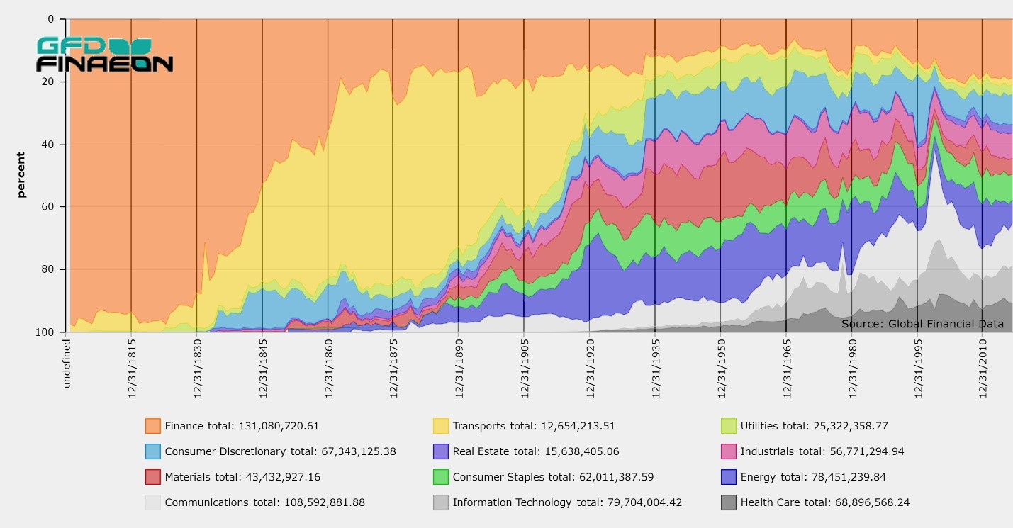
The GFD-100 Index is superior to existing indices for three reasons. First, the index is capitalization weighted from its beginning in 1791 until 2019. Second, the selection of stocks is based upon all shares that were traded on U.S. exchanges and over-the-counter. The selection of shares is not limited to the New York Stock Exchange (NYSE), but includes shares from regional exchanges and over-the-counter markets. Third, the index includes finance stocks throughout its history. Finance shares were excluded from the S&P 500 Composite until July 1, 1976 when the composition of the S&P 500 was changed from 425 Industrials, 60 Utilities and 15 Rail shares (adopted in March 1957) to 400 Industrials, 40 Utilities, 20 Transportation and 40 Finance stocks.
Few people realize that bank and insurance stocks were excluded from any major United States stock index until 1976. Although bank and finance stocks mostly traded over-the-counter before the 1970s, finance stocks represented between 10% and 20% of the overall capitalization of the stock market before 1976. Bank and insurance companies were excluded because consistent price quotes were not available and finance stocks were not as liquid as the shares traded on exchanges. The exclusion of over-the-counter shares was not limited to banks and insurance companies. Standard Oil and its subsidiaries also traded over-the-counter and were excluded from stock market indices until they moved onto the New York Stock Exchange. Nevertheless, people did invest in bank and insurance stocks, and in the Standard Oil companies, and their exclusion creates biases in the historical calculations of stock market indices.
Existing calculations of long-term stock market returns in the United States are based upon four primary sources: Smith and Cole (1803-1862), Macaulay (1857-1871) Cowles (1871-1928) and Standard and Poor’s (1928-2017). Unfortunately, these indices have major flaws in them that create biases that researchers have tolerated until now because no one has ever collected historical data on U.S. share prices, corporate actions (dividends and splits) and shares outstanding so accurate price and return indices could be calculated. The current S&P Composite includes data from the Cowles Indices from 1871 until 1927, the 90-share daily S&P Index from January 1928 until February 1957, the 500-share composite that excludes finance stocks until July 1976 and the all-sector 500-share index since July 1, 1976.
Global Financial Data has collected data on all major United States exchanges going back to 1791 as well as data on over-the-counter shares since 1865. The data includes not only share price data, but information on corporate actions (dividends and splits) as well as shares outstanding. These data sources enable us to calculate cap-weighted price and return indices for the United States that accurately reflect what an investment in the 100 largest stocks each year would have produced for investors.
GFD set up criteria for determining which stocks are included or excluded from its indices. GFD has followed these rules for inclusion: 1) there had to be at least 9 observations per year, 2) Dividend data have to be available for each stock in order that both price and return indices can be calculated, and 3) There had to be share outstanding information available so the stock could be included in a capitalization-weighted index.
The index includes all shares that met these criteria from 1791 to 1824, the top 50 shares by capitalization are used from 1825 to 1850 and the top 100 shares by capitalization from 1851 to 2017. To choose which companies to include, shares were weighted by capitalization during the first month of each year and included if they were among the 100 largest shares in the United States. It was assumed that the stocks were held for the rest of the year, and in January of the next year, the same selection methodology was used to choose which shares to hold for the coming year. Each year, the list of the 100 largest companies was recalculated and a new list of stocks was introduced. For continuity purposes, if a stock missed a year, i.e. the stock was in the top 100 in 1914 and 1916, but not in 1915, the stock was included in the index in 1915 even though this put over 100 stocks in the index.
Global Financial Data has calculated a 100-share index that is more comprehensive than existing long-term indices of the United States stock market. GFD has collected historical data on U.S. shares from 1791 until 2017 and is using this database to calculate a more representative index of U.S. shares than is currently available.
The GFD-100 Index is superior to existing indices for three reasons. First, the index is capitalization weighted from its beginning in 1791 until 2019. Second, the selection of stocks is based upon all shares that were traded on U.S. exchanges and over-the-counter. The selection of shares is not limited to the New York Stock Exchange (NYSE), but includes shares from regional exchanges and over-the-counter markets. Third, the index includes finance stocks throughout its history. Finance shares were excluded from the S&P 500 Composite until July 1, 1976 when the composition of the S&P 500 was changed from 425 Industrials, 60 Utilities and 15 Rail shares (adopted in March 1957) to 400 Industrials, 40 Utilities, 20 Transportation and 40 Finance stocks.
Few people realize that bank and insurance stocks were excluded from any major United States stock index until 1976. Although bank and finance stocks mostly traded over-the-counter before the 1970s, finance stocks represented between 10% and 20% of the overall capitalization of the stock market before 1976. Bank and insurance companies were excluded because consistent price quotes were not available and finance stocks were not as liquid as the shares traded on exchanges. The exclusion of over-the-counter shares was not limited to banks and insurance companies. Standard Oil and its subsidiaries also traded over-the-counter and were excluded from stock market indices until they moved onto the New York Stock Exchange. Nevertheless, people did invest in bank and insurance stocks, and in the Standard Oil companies, and their exclusion creates biases in the historical calculations of stock market indices.
Existing calculations of long-term stock market returns in the United States are based upon four primary sources: Smith and Cole (1803-1862), Macaulay (1857-1871) Cowles (1871-1928) and Standard and Poor’s (1928-2017). Unfortunately, these indices have major flaws in them that create biases that researchers have tolerated until now because no one has ever collected historical data on U.S. share prices, corporate actions (dividends and splits) and shares outstanding so accurate price and return indices could be calculated. The current S&P Composite includes data from the Cowles Indices from 1871 until 1927, the 90-share daily S&P Index from January 1928 until February 1957, the 500-share composite that excludes finance stocks until July 1976 and the all-sector 500-share index since July 1, 1976.
Global Financial Data has collected data on all major United States exchanges going back to 1791 as well as data on over-the-counter shares since 1865. The data includes not only share price data, but information on corporate actions (dividends and splits) as well as shares outstanding. These data sources enable us to calculate cap-weighted price and return indices for the United States that accurately reflect what an investment in the 100 largest stocks each year would have produced for investors.
GFD set up criteria for determining which stocks are included or excluded from its indices. GFD has followed these rules for inclusion: 1) there had to be at least 9 observations per year, 2) Dividend data have to be available for each stock in order that both price and return indices can be calculated, and 3) There had to be share outstanding information available so the stock could be included in a capitalization-weighted index.
The index includes all shares that met these criteria from 1791 to 1824, the top 50 shares by capitalization are used from 1825 to 1850 and the top 100 shares by capitalization from 1851 to 2017. To choose which companies to include, shares were weighted by capitalization during the first month of each year and included if they were among the 100 largest shares in the United States. It was assumed that the stocks were held for the rest of the year, and in January of the next year, the same selection methodology was used to choose which shares to hold for the coming year. Each year, the list of the 100 largest companies was recalculated and a new list of stocks was introduced. For continuity purposes, if a stock missed a year, i.e. the stock was in the top 100 in 1914 and 1916, but not in 1915, the stock was included in the index in 1915 even though this put over 100 stocks in the index.

| Decade | Stock Price | Stock Return | Dividends | Bonds | Cash | Equity Premium |
|---|---|---|---|---|---|---|
| 1792-1799 | -3.7 | 2.67 | 6.61 | -0.15 | 5.75 | -2.91 |
| 1800-1809 | 1.35 | 8.01 | 6.57 | 6.03 | 4.96 | 2.91 |
| 1810-1819 | -4.35 | 1.59 | 6.21 | 7.42 | 4.99 | -3.24 |
| 1820-1829 | 0.53 | 5.82 | 5.26 | 5.01 | 3.66 | 2.08 |
| 1830-1839 | -0.95 | 5 | 6.01 | 0.44 | 4.51 | 0.47 |
| 1840-1849 | -0.8 | 6.12 | 6.98 | 6.97 | 4.94 | 1.12 |
| 1850-1859 | -0.58 | 6.65 | 7.27 | 4.67 | 5.01 | 1.56 |
| 1860-1869 | 4.62 | 12.45 | 7.48 | 9.28 | 4.97 | 7.13 |
| 1870-1879 | 2.04 | 8.97 | 6.79 | 5.52 | 3.82 | 4.96 |
| 1880-1889 | 1.19 | 6.27 | 5.02 | 4.16 | 3.01 | 7.98 |
| 1890-1899 | 4.05 | 9.45 | 5.19 | 4.57 | 2.13 | 2.81 |
| 1900-1909 | 6.25 | 11.23 | 4.69 | 0.76 | 3.01 | 7.98 |
| 1910-1919 | -0.69 | 5.5 | 6.23 | 2.22 | 2.62 | 2.81 |
| 1920-1929 | 8.72 | 14.44 | 5.26 | 5.53 | 3.5 | 10.57 |
| 1930-1939 | -3.48 | 0.5 | 4.12 | 6.32 | 0.27 | 0.23 |
| 1940-1949 | 3.43 | 8.21 | 4.62 | 2.25 | 0.58 | 7.59 |
| 1950-1959 | 13.67 | 18.3 | 4.07 | 0.70 | 2.16 | 15.80 |
| 1960-1969 | 3.82 | 6.83 | 2.90 | 1.28 | 4.4 | 2.33 |
| 1970-1979 | 2.14 | 6.12 | 3.90 | 4.09 | 6.71 | -0.55 |
| 1980-1989 | 12.94 | 18.14 | 4.60 | 15.54 | 7.96 | 9.43 |
| 1990-1999 | 19.78 | 22.65 | 2.40 | 7.20 | 4.52 | 17.35 |
| 2000-2009 | -1.66 | 0.16 | 1.85 | 5.42 | 2.25 | -2.04 |
| 2010-2017 | 7.67 | 10.06 | 2.22 | 3.67 | 0.21 | 9.83 |
| Average | 3.30 | 8.48 | 5.06 | 4.73 | 3.74 | 4.60 |