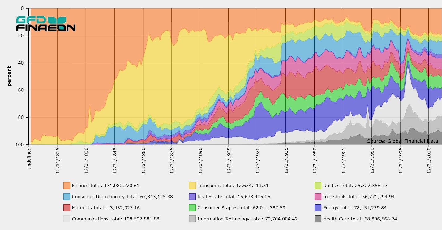
 The Dow Jones Industrial Average (DJIA) is both the oldest stock index for industrial stocks in the United States and a benchmark for stocks in the United States. When someone says “the market” was up 100 points today, they are referring to the Dow Jones Industrial Average. Most people are unaware of the history of the DJIA and that Global Financial Data’s provides a unique version of the DJIA that extends the series on a daily basis back to 1885 by combining all four versions of the DJIA into a single index, and provides data unavailable from any other data source. Global Financial Data is also the only source that provides data on all the historical components of the DJIA.
The Four Indices


Global Financial Data’s Version of the Dow Jones Industrial Average
GFD’s version of the DJIA includes several adjustments that are unique. First, we have combined the four versions of the DJIA into a single index by introducing adjustment factors when new indices were introduced in 1886, 1896 and 1914. We were able to accurately do this by going back to the New York Times in 1886 and 1896 to calculate the prices of the stocks in the new and the old averages on the day the new index was introduced. Once we found the ratio of stocks in the old and new Industrial indices we used this adjustment factor to chain link the series together.
The Dow Jones Industrial Average is the grandfather of stock market indices with a history stretching back to 1885, providing 125 years of daily data on US stocks. The index has been substantially revised 3 times by changing the number of stocks or components within the index.
GFD provides three unique features to help investors understand the history of the DJIA. First, we provide adjustment factors that enable users to chain link each of these indices together and provide a more complete picture of the DJIA and US stocks over time. By choosing the “Split Adjusted” choice in the Download Tool, the data will automatically adjust for these changes. Second, we have recreated the index during the NYSE’s closure in 1914 to provide our users information on US stocks unavailable anywhere else.

 Depending on who you ask, Interest rates will move up in the next 1 to 5 years. With this move in mind, it is necessary to look at the performance of some of the asset classes that could be affected by this move. In this graph you can see that falling interested rates are beneficial for preferred stock but when interest rates move up, their performance suffers.

 The Company of Proprietors of the Grand Junction Canal was incorporated by Special Act of Parliament on April 30, 1793 to build a canal from Braunston to the River Thames. The stock for the canal went through three bubbles, in the 1790s, the 1810s and the 1820s, before settling down once the railroads were built, providing competition to the canal.
Unfortunately, there is almost no data for the Canal Mania of the 1790s. The number of canals authorized by Act of Parliament in 1790 was one, but by 1793 twenty were authorized. The capital authorized in 1790 was £90,000, but had risen to £2,824,700 by 1793. Most of the canals raised their money locally, mainly in the Midlands, and there were few transactions in the stocks as a result. Though a stock exchange was established in Liverpool to trade shares, actual values are hard to come by and must be tracked down through newspapers. Nevertheless, some of the stock increases were impressive. The Birmingham and Fazeley showed the greatest increase, trading at a premium of £1170 in 1793.
The first bubble occurred in 1792 and 1793 and we only have two prices for Grand Junction Canal Shares, one at £472.75 in October 1792, a premium of 355 guineas, even before the company had started to dig the canal or gotten approval from Parliament! Talk about a speculative bubble. Shares had fallen to £441 by the time the approval was provided by Parliament, and the prices collapsed after 1795 when shares returned to their par level of around 100.
The Company of Proprietors of the Grand Junction Canal was incorporated by Special Act of Parliament on April 30, 1793 to build a canal from Braunston to the River Thames. The stock for the canal went through three bubbles, in the 1790s, the 1810s and the 1820s, before settling down once the railroads were built, providing competition to the canal.
Unfortunately, there is almost no data for the Canal Mania of the 1790s. The number of canals authorized by Act of Parliament in 1790 was one, but by 1793 twenty were authorized. The capital authorized in 1790 was £90,000, but had risen to £2,824,700 by 1793. Most of the canals raised their money locally, mainly in the Midlands, and there were few transactions in the stocks as a result. Though a stock exchange was established in Liverpool to trade shares, actual values are hard to come by and must be tracked down through newspapers. Nevertheless, some of the stock increases were impressive. The Birmingham and Fazeley showed the greatest increase, trading at a premium of £1170 in 1793.
The first bubble occurred in 1792 and 1793 and we only have two prices for Grand Junction Canal Shares, one at £472.75 in October 1792, a premium of 355 guineas, even before the company had started to dig the canal or gotten approval from Parliament! Talk about a speculative bubble. Shares had fallen to £441 by the time the approval was provided by Parliament, and the prices collapsed after 1795 when shares returned to their par level of around 100.

The London Stock Exchange wasn’t formally established until 1801, so until then the opportunity to trade canal stocks and keep track of the price fluctuations was limited. Even once the London Stock Exchange was established in 1801, most of the prices we have from the Gentlemen’s Magazine and other sources. The data are bid and ask quotes rather than actual prices since the shares still traded infrequently. Nevertheless, these data are sufficient to outline the three bubbles in shares of the Grand Junction Canal. The next price we have for Grand Junction Canal shares after 1793 is of £94 in April 1806. The bubble began in May 1808 when the shares still traded at £96, but the price steadily rose to £313.5 by June 1808, whence they declined to £179 by August 1811, stabilized around 200 until 1815 when the Napoleonic War ended, then fell to £103 by September 1816. The second Canal Mania of the 1810s was not as wild as the one of the 1790s, since share prices tripled rather than quadrupled, but the difference was that the Canal Mania of the 1810s was not limited to the Midlands. Shareholders in London also participated as a result of the establishment of the Stock Exchange.

Bubbles require both a source for the speculation, a new technology that excites investors and causes cash to quickly flow into the new discovery, and excess credit being made available to invest in the shares. The initial canal mania was driven by profits with one canal paying a £75 dividend. Many of the stocks were profitable, and did quite well, but others that were poorly thought out failed. The two bubbles that drove Grand Junction Canal shares in the 1810s and 1820s were driven not only by the investment opportunities the canals provided, but by the liquidity created by the impact of the Napoleonic Wars on Britain finances.
 With Google and Priceline surpassing $1000 (much less Berkshire Hathaway A shares trading at $175,000), people are amazed that stocks can trade at such high levels without being overvalued or losing liquidity, but in reality, compared with the past, most stocks are cheap nowadays. In fact, the further you go back in time, the higher was the price of average stocks to most investors. In terms of purchasing power, stocks are as cheap and as liquid as they have ever been.
Not only was the average price of stocks 200 years higher than they are today, but they were higher in terms of personal income. Shares of the First Bank of the United States were issued at $400 in 1791 and shares of the Massachusetts Bank of Boston were issued at $500 in 1792. One share was equivalent to the average annual income of most people back then. Most shares sold for $100, and some for $50 or $25, so how could investors afford stocks that make Google and Priceline look cheap? Even if a stock was at $100, this was equivalent to $10,000 today in terms of earning power. Were there really that many rich people back then? The answer is no, but the difference is in the way shares were issued and traded.
First, shares were rarely bought in round lots of 100 shares as they are today, but shares were traded individually. This means that even though the prices of individual shares has fallen, the average transaction size has not fallen as significantly.
Second, and most importantly, shares were often bought on the installment plan, at a discount, or in fractions in order to reduce the total cost of investing. It is this second point I want to concentrate on.
To see how this worked, let’s go back to the South Sea Bubble of 1720. It should be remembered that South Sea shares traded around £100 before the bubble began, which was equivalent to about $500 in 1720. One factor that allowed the Bubble to occur was that “investors” were allowed to pay for their shares in installments. The initial purchase required only 10% down with the rest of the payments spread over the rest of 1720. This was the eighteenth-century version of buying on margin. It encouraged buying because speculators, as always, thought they could make a profit before the next payment was due. It was the eighteenth-century equivalent of flipping houses. Many of them, no doubt, knew they didn’t have the full amount of money for a share, but they did have enough to get in the game. Unfortunately, the game got them.
Without the speculative allure of buying in down payments, trading remained quiet in London for the next 100 years. Speculation only returned during the Canal Bubble of the 1810s, the South America and Mining boom of the 1820s and the railroad boom of the 1840s. The difference between how stocks traded in the 1840s and today is particularly striking. Again, the difference is what I call, buying on the installment plan.
The par value of most stocks was £100 or about $486 using the fixed, gold exchange rate. This was almost a year’s income for the average person. Of course, the average person wasn’t investing, and most investors were people who had an endowment they had to live off of. The problem was, if you want to build a railroad and raise large amounts of money, how do you get people to part with their money? As in 1720, the answer was to pay on the installment plan.
A railroad stock would be issued at £100 par. This was the amount investors were expected to put into the company; however, the company would only ask for the money as needed. The amount actually paid in was the Paid amount, and this could differ significantly from the par value. The agreement was that as the building of the railroad progressed, the corporation could assess shareholders for additional money, which they would then be required to pay in, or lose their shares. This allowed shareholders to get in on the cheap and spread out their £100 in payments over a period of several years, starting off at £10 and working their way up. As always, the hope was that if the railroad were successful, investors could use the profits to pay for the shares, and if the railroad were not successful, this process would minimize their losses. In theory, after several years, the £100 would be paid in full, and the shareholder would have made a successful investment.
In reality, this created a number of complications. First, there was always the problem that someone might not have the cash ready when an assessment was due. For this reason, shareholders began to resent the fact that at any point in time the corporation could ask them for more money with the threat of the loss of shares if the shareholder did not pay. The goal was to receive money from the corporation, not pay money into it. Shareholders especially resented this when the railroad ran into unexpected problems creating a need for the investors to share the burden. It is one thing to lose money on a stock; it is another to have to pay money into the company in addition to losing your capital. This is why all shares today are non-assessable, meaning companies cannot ask shareholders for more money.
The oddest result of this system was that some shares might actually trade at a negative value! In other words, someone would pay you to take their shares in the company, and we have recorded negative values for shares from the London SE. Let’s say that a share is trading at £5 and a £10 assessment is due, but you don’t have the £10, then you might pay someone £5 to take the shares off your hands and avoid the £10 assessment. Having to pay someone to take shares of a company you invested and lost money on would certainly add insult to injury.
Another problem this system created was that several shares could trade simultaneously. You might have shares with £30, £40 and £50 trading at the same time reflecting the amount paid in and creating confusion. For this reason, prices were often quoted in the London Times at a premium or discount to the par value, so the same amount would be paid regardless of which shares you were buying. So if the shares were trading at a £5 discount, you would pay £25 for the £30 shares or £35 for the £40 shares. Up until the mid-nineteenth century, most shares on the London Stock Exchange that were not at their fully paid value were listed this way.
There was another problem this created. When the railroad boom got going in the 1840s, stocks increased in value dramatically. If a railroad needed to raise more capital, and the shares were already fully paid in at 100 and had risen in price since then because the railroad was profitable, it became difficult to raise additional capital because the price of the shares was so high. So how do you raise additional capital? The answer was simple, you issue fractional shares.
Shares were issued in halves, thirds, fourths, fifths, eighths, tenths, sixteenths, and most points in between. At any given point, a company might have a half-dozen fractional shares issued and trading. This allowed smaller investors to jump on the bandwagon and make money along with their richer friends. In addition to this, the railroad might issue shares specifically for specific routes along the railroad which would be separate from the main line. This allowed the railroad to issue new shares at lower prices on the installment plan, and since money is fungible, use the money as they best saw fit.
Of course, most shareholders wanted to receive income on their shares in the form of dividends. After the railroad mania of the 1840s was over with, profits were lower and shares had declined in value. It became more difficult to raise money from this sector of the investing public, so some of the railroads began issuing “preferred” shares which were paid ahead of the common stocks. In fact, it was the London and Greenwich Railway which was the first to do this, issuing a 5% preferred in April 1842.
By the time the railway mania of the 1840s was over, the result was that the outstanding securities of some railroads were a mess. Most railroads never made it to the full £100 paid in, so the paid in value was only a portion of their par value. In addition to that, fractional shares were outstanding, and there were the shares from extension lines of the railroad as well as shares in railroads taken over during the boom, which usually traded separately from the parent shares.
To eliminate the confusion, railroads consolidated shares once the building boom was over with. If a £100 par share was at £20 paid, the company would do a 1:5 reverse split turning the stock into a £100 par share. If there were half shares or quarter shares outstanding, they would do a 1:10 or 1:20 reverse so all the fractional shares were eliminated. If an extension rail line was at £10 par, it would have a 1:10 reverse. Consequently, all the shares would be consolidated into a single security.
By the late 1800s, capital was flowing freely enough that all the measures that had been used to make shares “affordable” were no longer needed, and new shares were issued at £100 and the whole system of downpayments, fractional shares, and other half-measures weren’t necessary anymore.
Nevertheless, there was a final interesting phenomenon which occurred in London to make shares more accessible to the public. When the bull market of the 1920s occurred, the high price of stocks kept most shareholders out of the market, even though punters wanted in. Companies found a quick solution to making their shares more liquid and bringing in more capital.
In the US, companies would split their stocks 4:1 or 5:1 as the price rose to make the shares more affordable, and speculators could go to bucket shops to trade on margin, but in London, shares were sometimes split 100:1 to get the par value down from £100 to £1, and there are even cases of stocks splitting 400:1 to get the par value down to 5 shillings (or about $1). This helped to feed the bull market in stocks in London, but as we all know, the 1920s bull market ended in the crash of the Great Depression, though stocks fell around 50% in London, as opposed to 90% in the United States.
The bottom line is, companies will always find a way to make their shares available to the public to raise money and maintain liquidity in their stocks. Some may criticize high-frequency trading, but it has made the markets more liquid. It is easier and cheaper to trade odd lots than ever, so if you only want to buy 10 shares of Google, then do so. Markets have always accommodated investors, and always will.
With Google and Priceline surpassing $1000 (much less Berkshire Hathaway A shares trading at $175,000), people are amazed that stocks can trade at such high levels without being overvalued or losing liquidity, but in reality, compared with the past, most stocks are cheap nowadays. In fact, the further you go back in time, the higher was the price of average stocks to most investors. In terms of purchasing power, stocks are as cheap and as liquid as they have ever been.
Not only was the average price of stocks 200 years higher than they are today, but they were higher in terms of personal income. Shares of the First Bank of the United States were issued at $400 in 1791 and shares of the Massachusetts Bank of Boston were issued at $500 in 1792. One share was equivalent to the average annual income of most people back then. Most shares sold for $100, and some for $50 or $25, so how could investors afford stocks that make Google and Priceline look cheap? Even if a stock was at $100, this was equivalent to $10,000 today in terms of earning power. Were there really that many rich people back then? The answer is no, but the difference is in the way shares were issued and traded.
First, shares were rarely bought in round lots of 100 shares as they are today, but shares were traded individually. This means that even though the prices of individual shares has fallen, the average transaction size has not fallen as significantly.
Second, and most importantly, shares were often bought on the installment plan, at a discount, or in fractions in order to reduce the total cost of investing. It is this second point I want to concentrate on.
To see how this worked, let’s go back to the South Sea Bubble of 1720. It should be remembered that South Sea shares traded around £100 before the bubble began, which was equivalent to about $500 in 1720. One factor that allowed the Bubble to occur was that “investors” were allowed to pay for their shares in installments. The initial purchase required only 10% down with the rest of the payments spread over the rest of 1720. This was the eighteenth-century version of buying on margin. It encouraged buying because speculators, as always, thought they could make a profit before the next payment was due. It was the eighteenth-century equivalent of flipping houses. Many of them, no doubt, knew they didn’t have the full amount of money for a share, but they did have enough to get in the game. Unfortunately, the game got them.
Without the speculative allure of buying in down payments, trading remained quiet in London for the next 100 years. Speculation only returned during the Canal Bubble of the 1810s, the South America and Mining boom of the 1820s and the railroad boom of the 1840s. The difference between how stocks traded in the 1840s and today is particularly striking. Again, the difference is what I call, buying on the installment plan.
The par value of most stocks was £100 or about $486 using the fixed, gold exchange rate. This was almost a year’s income for the average person. Of course, the average person wasn’t investing, and most investors were people who had an endowment they had to live off of. The problem was, if you want to build a railroad and raise large amounts of money, how do you get people to part with their money? As in 1720, the answer was to pay on the installment plan.
A railroad stock would be issued at £100 par. This was the amount investors were expected to put into the company; however, the company would only ask for the money as needed. The amount actually paid in was the Paid amount, and this could differ significantly from the par value. The agreement was that as the building of the railroad progressed, the corporation could assess shareholders for additional money, which they would then be required to pay in, or lose their shares. This allowed shareholders to get in on the cheap and spread out their £100 in payments over a period of several years, starting off at £10 and working their way up. As always, the hope was that if the railroad were successful, investors could use the profits to pay for the shares, and if the railroad were not successful, this process would minimize their losses. In theory, after several years, the £100 would be paid in full, and the shareholder would have made a successful investment.
In reality, this created a number of complications. First, there was always the problem that someone might not have the cash ready when an assessment was due. For this reason, shareholders began to resent the fact that at any point in time the corporation could ask them for more money with the threat of the loss of shares if the shareholder did not pay. The goal was to receive money from the corporation, not pay money into it. Shareholders especially resented this when the railroad ran into unexpected problems creating a need for the investors to share the burden. It is one thing to lose money on a stock; it is another to have to pay money into the company in addition to losing your capital. This is why all shares today are non-assessable, meaning companies cannot ask shareholders for more money.
The oddest result of this system was that some shares might actually trade at a negative value! In other words, someone would pay you to take their shares in the company, and we have recorded negative values for shares from the London SE. Let’s say that a share is trading at £5 and a £10 assessment is due, but you don’t have the £10, then you might pay someone £5 to take the shares off your hands and avoid the £10 assessment. Having to pay someone to take shares of a company you invested and lost money on would certainly add insult to injury.
Another problem this system created was that several shares could trade simultaneously. You might have shares with £30, £40 and £50 trading at the same time reflecting the amount paid in and creating confusion. For this reason, prices were often quoted in the London Times at a premium or discount to the par value, so the same amount would be paid regardless of which shares you were buying. So if the shares were trading at a £5 discount, you would pay £25 for the £30 shares or £35 for the £40 shares. Up until the mid-nineteenth century, most shares on the London Stock Exchange that were not at their fully paid value were listed this way.
There was another problem this created. When the railroad boom got going in the 1840s, stocks increased in value dramatically. If a railroad needed to raise more capital, and the shares were already fully paid in at 100 and had risen in price since then because the railroad was profitable, it became difficult to raise additional capital because the price of the shares was so high. So how do you raise additional capital? The answer was simple, you issue fractional shares.
Shares were issued in halves, thirds, fourths, fifths, eighths, tenths, sixteenths, and most points in between. At any given point, a company might have a half-dozen fractional shares issued and trading. This allowed smaller investors to jump on the bandwagon and make money along with their richer friends. In addition to this, the railroad might issue shares specifically for specific routes along the railroad which would be separate from the main line. This allowed the railroad to issue new shares at lower prices on the installment plan, and since money is fungible, use the money as they best saw fit.
Of course, most shareholders wanted to receive income on their shares in the form of dividends. After the railroad mania of the 1840s was over with, profits were lower and shares had declined in value. It became more difficult to raise money from this sector of the investing public, so some of the railroads began issuing “preferred” shares which were paid ahead of the common stocks. In fact, it was the London and Greenwich Railway which was the first to do this, issuing a 5% preferred in April 1842.
By the time the railway mania of the 1840s was over, the result was that the outstanding securities of some railroads were a mess. Most railroads never made it to the full £100 paid in, so the paid in value was only a portion of their par value. In addition to that, fractional shares were outstanding, and there were the shares from extension lines of the railroad as well as shares in railroads taken over during the boom, which usually traded separately from the parent shares.
To eliminate the confusion, railroads consolidated shares once the building boom was over with. If a £100 par share was at £20 paid, the company would do a 1:5 reverse split turning the stock into a £100 par share. If there were half shares or quarter shares outstanding, they would do a 1:10 or 1:20 reverse so all the fractional shares were eliminated. If an extension rail line was at £10 par, it would have a 1:10 reverse. Consequently, all the shares would be consolidated into a single security.
By the late 1800s, capital was flowing freely enough that all the measures that had been used to make shares “affordable” were no longer needed, and new shares were issued at £100 and the whole system of downpayments, fractional shares, and other half-measures weren’t necessary anymore.
Nevertheless, there was a final interesting phenomenon which occurred in London to make shares more accessible to the public. When the bull market of the 1920s occurred, the high price of stocks kept most shareholders out of the market, even though punters wanted in. Companies found a quick solution to making their shares more liquid and bringing in more capital.
In the US, companies would split their stocks 4:1 or 5:1 as the price rose to make the shares more affordable, and speculators could go to bucket shops to trade on margin, but in London, shares were sometimes split 100:1 to get the par value down from £100 to £1, and there are even cases of stocks splitting 400:1 to get the par value down to 5 shillings (or about $1). This helped to feed the bull market in stocks in London, but as we all know, the 1920s bull market ended in the crash of the Great Depression, though stocks fell around 50% in London, as opposed to 90% in the United States.
The bottom line is, companies will always find a way to make their shares available to the public to raise money and maintain liquidity in their stocks. Some may criticize high-frequency trading, but it has made the markets more liquid. It is easier and cheaper to trade odd lots than ever, so if you only want to buy 10 shares of Google, then do so. Markets have always accommodated investors, and always will.